Cell-wise analyses: indepth analyses of Pu.1 and GATA1 interactions

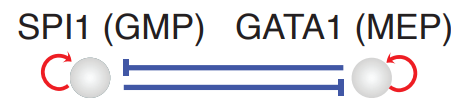
To obtain deep mechanistic insights into key regulatory motifs (such as the Pu.1/SPI1-Gata1 network motif, see the figure below) from different perspectives, we developed three complementary strategies: cell-wise, trajectory-wise and plane-wise analyses. In this tutorial, we will focus on analyzing the canonical SPI1-GATA1 network motif that play key roles in the bifurcation of GMP and MEP lineage. Specifically, we will guide you through a series of cell-wise regulatory network analyses.

Let us first import relevant packages and load the processed hematopoiesis adata object for scNT-seq HSC experiment reported in the dynamo Cell paper:

import numpy as np
import pandas as pd
import matplotlib.pyplot as plt

import sys
import os

import dynamo as dyn
import seaborn as sns

dyn.dynamo_logger.main_silence()

adata_labeling = dyn.sample_data.hematopoiesis()

Three approaches for in-depth network motif characterizations

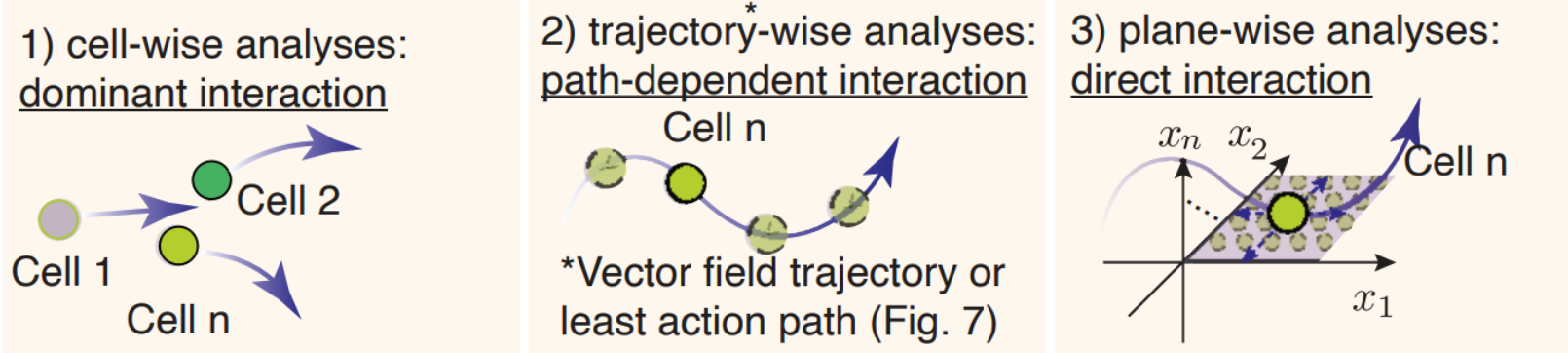
Here we will use a cartoon to explain the three complementary network analyses empowered by dynamo.

Cell-wise analyses to reveal dominant interactions across all cells

#. Trajectory-wise analyses reveal trajectory dependent interactions along a trajectory (predicted either from vector field streamline, or least action path, see Figure 6). #. Plane-wise analyses reveal direct interactions for any characteristic cell states by varying genes of interest while holding all other genes constant.

At this moment, we will focus on cell-wise analyses, the most common network interaction to analyze PU.1/SPI1–GATA1 network motif. Come back to check new tutorials on trajectory-wise and plane-wise analyses!

Cell-wise analyses of the PU.1/SPI1–GATA1 network motif across all cells

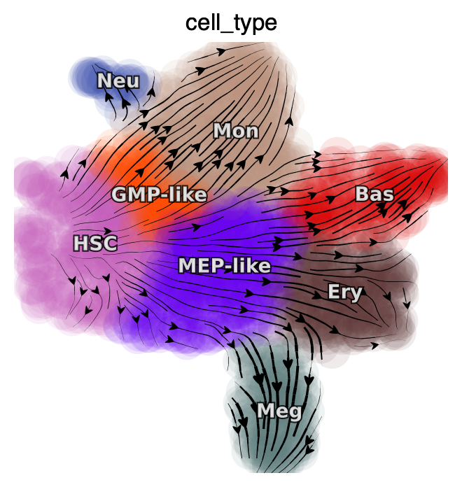
We will first plot the streamlines of SPI1 and GATA1 on UMAP space and while also color each cell based on their gene expression level.

dyn.pl.streamline_plot(
    adata_labeling,
    color=["cell_type"],
    layer="M_t",
    figsize=(4, 4),
    ncols=2
)

dyn.pl.streamline_plot(
    adata_labeling,
    color=["SPI1", "GATA1"],
    layer="M_t",
    figsize=(8, 4),
    ncols=2
)

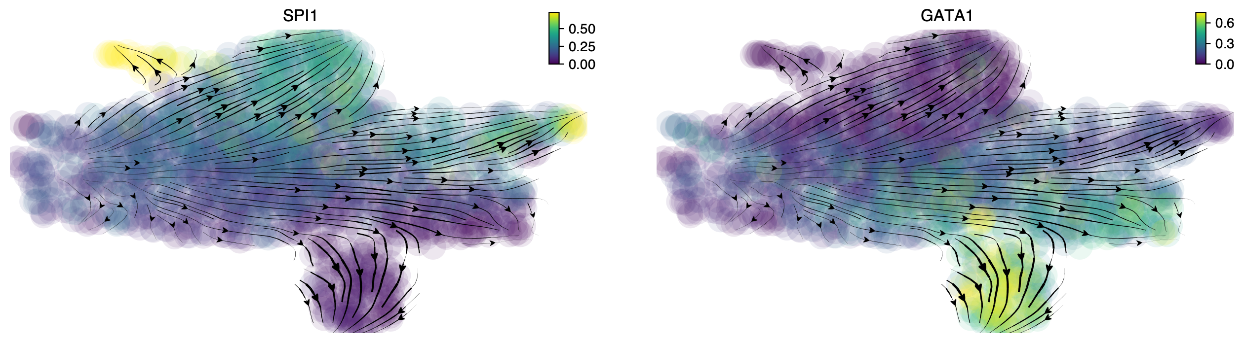
It is clear that SPI1 and GATA1’s gene expression shows high expression in GMP and MEP lineage, respectively, revealing a mutual exclusive expression pattern, as previously reported.

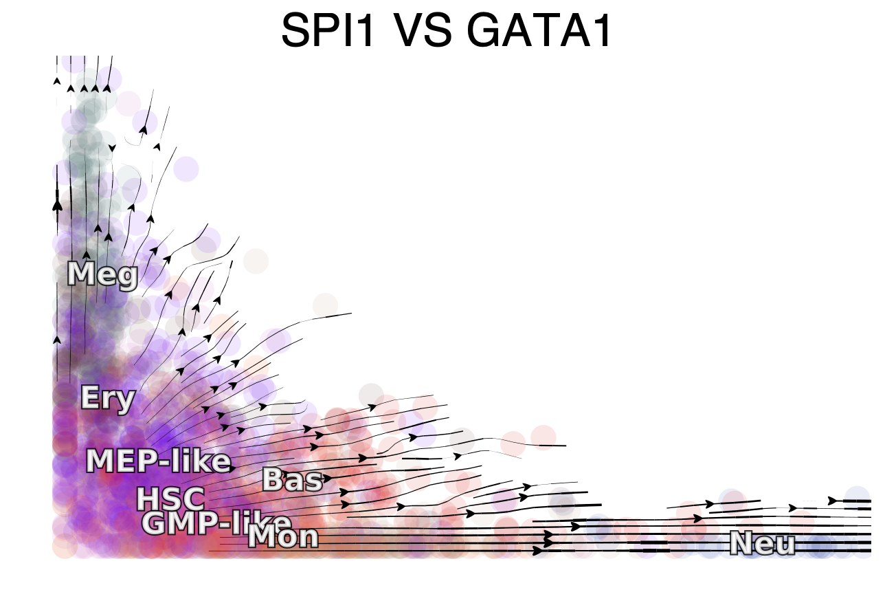
We next showcase the streamline plot of the RNA velocities of SPI1 (x-axis) and GATA1 (y-axis). Intriguingly, similar to decades of modeling efforts in simulating the vector field of Pu.1 and Gata1. The RNA velocity streamlines of SPI1 and GATA1 measured from real single cell data reveal nicely a bifurcation from HSPCs first to MEP or GMP like cells, followed by committing toward Ery/Meg lineages on the one side and Mon/Neu on the other hand. Interesting, the Bas lineage is located in the between between the two branching, indicating again, a potential dual origin from both GMP-like and MEP-like progenitors. This is very neat!!!

dyn.configuration.set_pub_style(scaler=4)
dyn.pl.streamline_plot(
    adata_labeling,
    color="cell_type",
    x="SPI1",
    y="GATA1",
    layer="M_t",
    ekey="M_t",
    pointsize=0.5,
    figsize=(8, 5),
    vkey="velocity_alpha_minus_gamma_s",
)

Next we will use jacobian to all pair-wise interactions between SPI1 and GATA1: #. Repression from SPI1 to GATA1, GATA1 to SPI1 #. Self-activation of SPI1, and GATA1.

In particular, we reveal the Jacobian in each cell on the SPI1 and GATA1 gene expression space (instead of the umap space):

%matplotlib inline

genes = ["SPI1", "GATA1"]
def plot_jacobian_on_gene_axis(receptor, effector, x_gene=None, y_gene=None, axis_layer="M_t", temp_color_key="temp_jacobian_color", ax=None):
    if x_gene is None:
        x_gene = receptor
    if y_gene is None:
        y_gene = effector

    x_axis = adata_labeling[:, x_gene].layers[axis_layer].A.flatten(),
    y_axis = adata_labeling[:, y_gene].layers[axis_layer].A.flatten(),

    dyn.vf.jacobian(adata_labeling, regulators = [receptor, effector], effectors=[receptor, effector])
    J_df = dyn.vf.get_jacobian(
        adata_labeling,
        receptor,
        effector,
    )
    color_values = np.full(adata_labeling.n_obs, fill_value=np.nan)
    color_values[adata_labeling.obs["pass_basic_filter"]] =  J_df.iloc[:, 0]
    adata_labeling.obs[temp_color_key] = color_values

    ax = dyn.pl.scatters(
        adata_labeling,
        vmin=0,
        vmax=100,
        color=temp_color_key,
        cmap="bwr",
        sym_c=True,
        frontier=True,
        sort="abs",
        alpha=0.1,
        pointsize=0.1,
        x=x_axis,
        y=y_axis,
        save_show_or_return="return",
        despline=True,
        despline_sides=["right", "top"],
        deaxis=False,
        ax=ax,
    )
    ax.set_title(r"$\frac{\partial f_{%s}}{\partial x_{%s}}$" % (effector, receptor))
    ax.set_xlabel(x_gene)
    ax.set_ylabel(y_gene)
    adata_labeling.obs.pop(temp_color_key)

figure, axes = plt.subplots(1, 4, figsize=(15, 3))
plot_jacobian_on_gene_axis("GATA1", "SPI1", x_gene="SPI1", y_gene="GATA1", ax=axes[0])
plot_jacobian_on_gene_axis("SPI1", "GATA1", x_gene="GATA1", y_gene="SPI1", ax=axes[1])
plot_jacobian_on_gene_axis("SPI1", "SPI1", x_gene="SPI1", y_gene="GATA1", ax=axes[2])
plot_jacobian_on_gene_axis("GATA1", "GATA1", x_gene="GATA1", y_gene="SPI1",ax=axes[3])
plt.show()

Transforming subset Jacobian: 100%|██████████| 1947/1947 [00:00<00:00, 127121.88it/s]
Transforming subset Jacobian: 100%|██████████| 1947/1947 [00:00<00:00, 124848.03it/s]
calculating Jacobian for each cell: 100%|██████████| 1947/1947 [00:00<00:00, 153429.97it/s]
calculating Jacobian for each cell: 100%|██████████| 1947/1947 [00:00<00:00, 183195.59it/s]

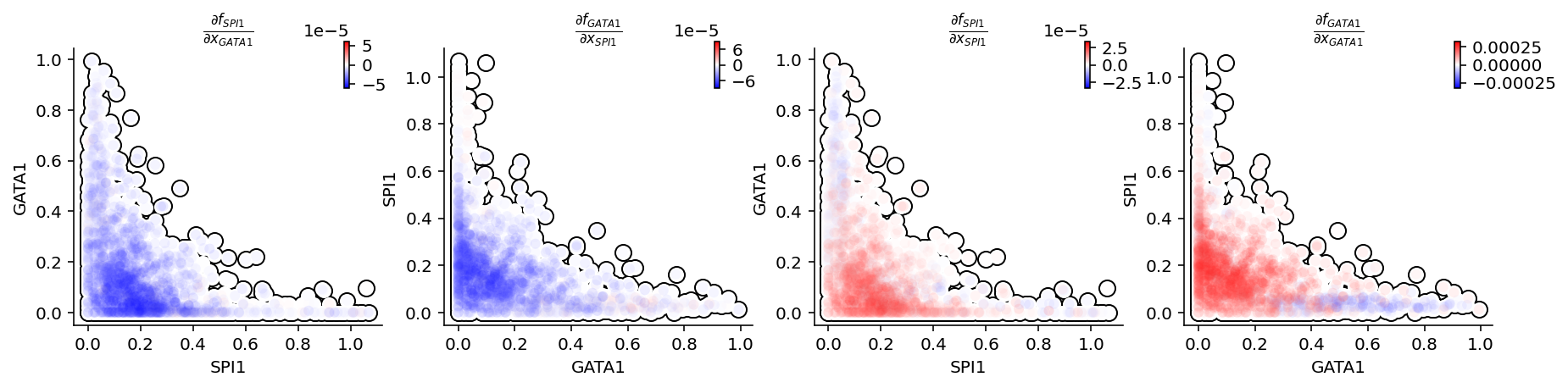
Looking close at the figure, we can immediately appreciate that the repression from SPI1 to GATA1 is mostly discernible in progenitors (rectangle A: bottom left) but becomes negligible when either GATA1 is much higher than SPI1 (rectangle B: upper left) or GATA1 is close to zero (rectangle C: bottom right). In contrast to the often assumed symmetrical regulation between Pu.1 and Gata 1. These results elucidate asymmetrical regulations within this canonical network motif. These results really highlights dynamo’s power in revealing novel mechanistic insights directly with the single cell genomics dataset. This is so cool!

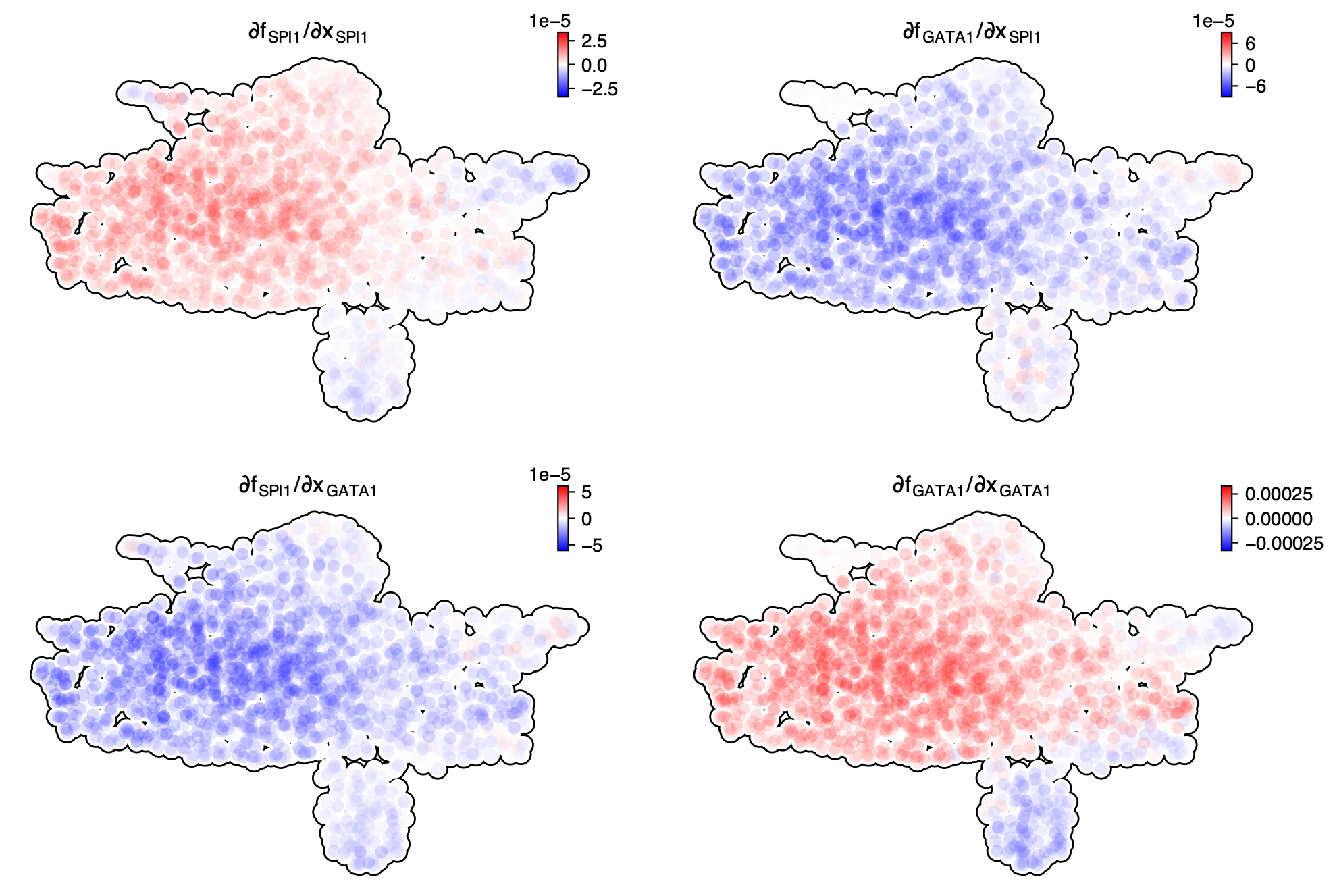
Similarly, we can also plot the Jacobian between SPI1 and GATA1 in the UMAP space, which again reveals their self-activation and mutual inhibition.

dyn.vf.jacobian(adata_labeling, regulators = ["SPI1", "GATA1"])
dyn.pl.jacobian(adata_labeling, regulators = ["SPI1", "GATA1"])

Transforming subset Jacobian: 100%|██████████| 1947/1947 [00:00<00:00, 127544.78it/s]

Response heatmap

To extract quantitative insights about the regulatory functions, we next plotted distributions of the four Jacobian elements versus expression of each gene with the so-called response heatmap, adapted from Scribe (Qiu et al., 2020b).

%matplotlib inline

dyn.vf.jacobian(adata_labeling, regulators=["SPI1", "GATA1"], effectors=["SPI1", "GATA1"])
dyn.pl.response(
    adata_labeling,
    np.array([["SPI1", "GATA1"], ["GATA1", "SPI1"], ["SPI1", "SPI1"], ["GATA1", "GATA1"]]),
    ykey="jacobian",
    log=False,
    drop_zero_cells=True,
    grid_num=25,
    figsize=(5, 3),
    save_show_or_return="show"
)

Transforming subset Jacobian: 100%|██████████| 1947/1947 [00:00<00:00, 125048.77it/s]

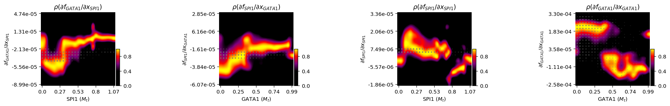
Interestingly, we found that the repression from SPI1 to GATA1 has a U shape with a clear valley while the repression from GATA1 to SPI1 is linear with the highest repression when GATA1 is very low. Similarly, the self-activation of SPI1 has a peak while that of GATA1 is linear. These results again reveal an asymmetrical regulation between PU.1 and GATA1.

Conclusion

In the analyses above, we illustrate how to use dynamo to perform various “cell-wise” analysis to explore different aspects of a regulatory network motif, such as the canonical PU.1/SPI1-GATA1 network motif as demonstrated here. A very nice result from our analyses is that we reveal asymmetrical instead of previously assumed symmetrical regulations between PU.1 and GATA1. Functionally, in the context of HSPC differentiation, where GATA1 has an overall lower initial expression in HSPCs than SPI1, the GATA1-SPI1 asymmetry may contribute to balanced lineage development. Given the high levels of SPI1 in HSPCs and the fact that knockdown of SPI1 to 20% of its original expression still allows emergence of GMP lineage, the low threshold of GATA1 for self-activation and inhibition to SPI1 helps it to compete with SPI1 to generate the MEP lineage.