Primer on differential geometry

In this work, we introduced dynamical systems theory and differential geometry analysis to single-cell genomics. A dynamical system describes the time dependence of points in a geometrical space, e.g., planetary motion or cell fate transitions, whereas differential geometry uses the techniques of differential/integral calculus and linear/multilinear algebra to study problems in geometry, e.g., the topology or geometric features along a streamline in vector field of the gene expression space.

A vector field function \(\mathbf{f}\), a fundamental topic of dynamical systems theories, takes spatial coordinate input \(\mathbf{x}\) (e.g., single-cell expression in gene state space) in a high-dimensional space (each gene corresponds to a dimension) as input and outputs a vector \(\mathbf v\) (e.g., corresponds to gene expression velocity vector from a single cell) in the same space, i.e. \(\mathbf v = \mathbf f(\mathbf x)\). In this study, we specifically discuss velocity vector fields that can be used to derive acceleration and curvature vector fields (see below). With analytical velocity vector field functions, including the ones that we learned directly from data, we can move beyond velocity to high-order quantities, including the Jacobian, divergence, acceleration, curvature, curl, etc., using theories developed in differential geometry. The discussion of the velocity vector field in this study focuses on transcriptomic space; vector fields, however, can be generally applicable to other spaces, such as morphological, proteomic, or metabolic space.

Because \(\mathbf f\) is a vector-valued multivariate function, a \(d\times d\) matrix encoding its derivatives, called the Jacobian, plays a fundamental role in differential geometry analysis of vector fields:

\[\begin{split}\begin{align*} \mathbf J &= \begin{bmatrix} &\dfrac{\partial f_1}{\partial x_1} & \dfrac{\partial f_1}{\partial x_2} & \cdots & \dfrac{\partial f_1}{\partial x_d} &\ \\[3ex] &\dfrac{\partial f_2}{\partial x_1} & \dfrac{\partial f_2}{\partial x_2} & \cdots & \dfrac{\partial f_2}{\partial x_d} &\ \\[1.5ex] &\vdots & \vdots & \ddots & \vdots &\ \\[1.5ex] &\dfrac{\partial f_d}{\partial x_1} & \dfrac{\partial f_d}{\partial x_2} & \cdots & \dfrac{\partial f_d}{\partial x_d} &\ \end{bmatrix} \ . \end{align*}\end{split}\]

A Jacobian element \(\partial f_i/\partial x_j\) reflects how the velocity of \(x_i\) is impacted by changes in \(x_j\).

Box Fig. 1. Divergence, curl, acceleration and curvature of vector field.

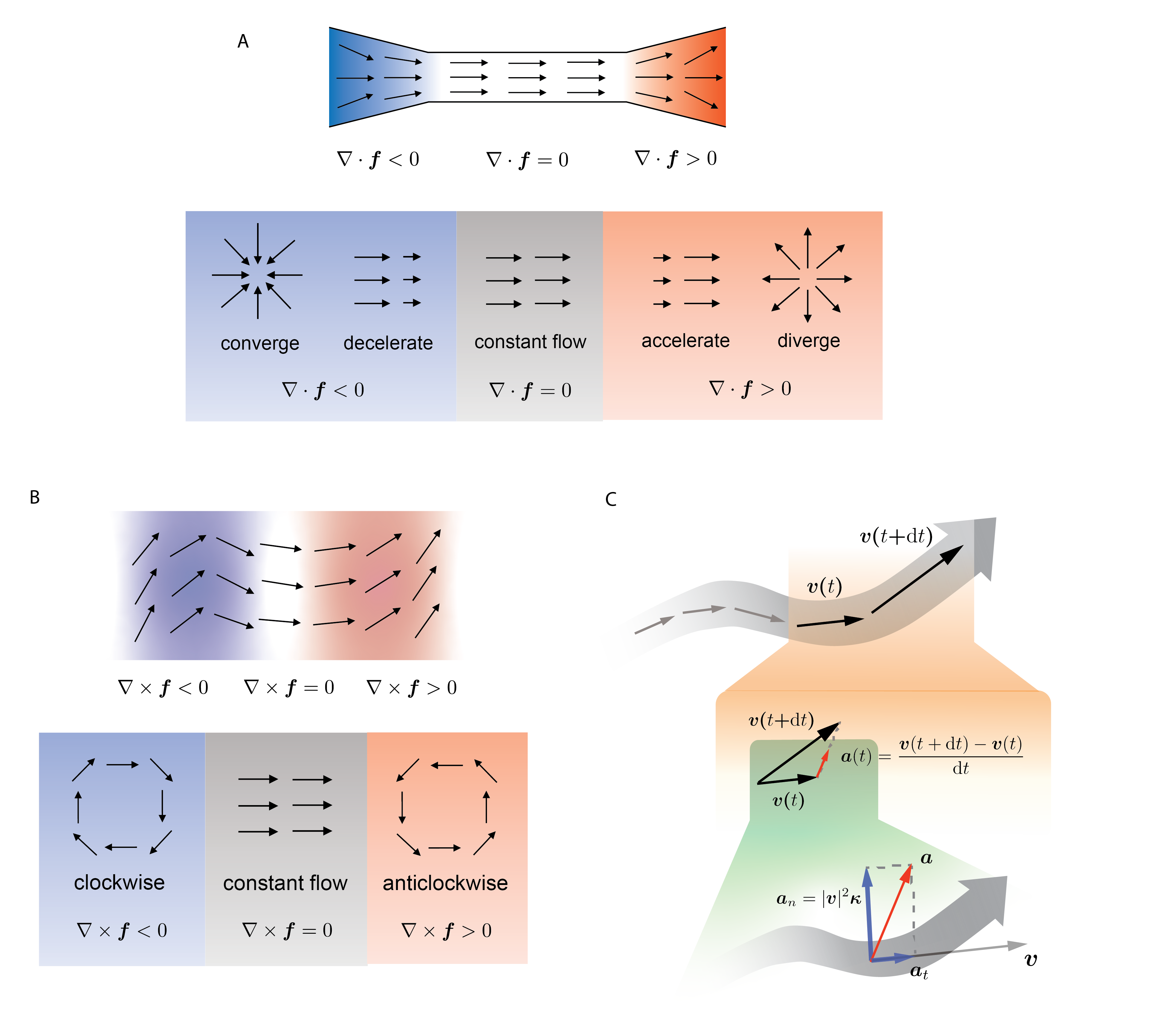
The trace of the Jacobian is divergence: \(\begin{align*} \nabla \cdot \mathbf f = \sum_{i=1}^{d}\dfrac{\partial f_i}{\partial x_i} = \mathrm{tr} \mathbf J \ . \end{align*}\)

Divergence measures the degree of “outgoingness” at any point, summarized in Box Fig. 1A.

By definition, an attractor (repulsor) converges (diverges) in any direction. Note that it is possible to have a point where the vectors converge in one direction but diverge in another, a case that is not depicted in the diagram above. This means that although an attractor (repulsor) always has negative (positive) divergence, the opposite does not necessarily hold.

Curl is a quantity measuring the degree of rotation at a given point in the vector field. It is well-defined only in two or three dimensions (e.g. two or three reduced principal components or UMAP components):

\[\begin{split}\begin{align*} \nabla \times \mathbf f &= \begin{bmatrix} \dfrac{\partial f_z}{\partial y} - \dfrac{\partial f_y}{\partial z} \\[2.5ex] \dfrac{\partial f_x}{\partial z} - \dfrac{\partial f_z}{\partial x} \\[2.5ex] \dfrac{\partial f_y}{\partial x} - \dfrac{\partial f_x}{\partial y} \end{bmatrix}\ . \end{align*}\end{split}\]

The behavior of curl is summarized in Box Fig. 1B.

Many differential geometry quantities are defined on streamlines. which are curves everywhere tangent to the vector field. The streamlines can be parametrized with time \(t\), denoted \(\mathbf x(t)\), as they are essentially trajectories of cells moving in the vector field. In practice, they are often calculated using numerical integration methods, e.g., the Runge–Kutta algorithm. The acceleration is the time derivative of the velocity, as shown in Box Fig. 1C (orange shade), and can be defined as:

\[\begin{align*} \mathbf a = \dfrac{\mathrm d \mathbf v}{\mathrm d t} = \dfrac{\mathrm d}{\mathrm d t}\mathbf f\Big(\mathbf x(t)\Big) = \sum_{i=1}^{d} \dfrac{\partial \mathbf f}{\partial x_i}\dfrac{\partial x_i}{\partial t} = \mathbf J \mathbf v \ . \end{align*}\]

The curvature vector (Box Fig. 1C, green shade) of a curve is defined as the derivative of the unit tangent vector (\(\frac{\mathrm d}{\mathrm dt}\frac{\mathrm v}{|\mathrm v|}\)), divided by the length of the tangent (\(|\mathrm v|\)):

\[\begin{align*} \mathrm \kappa = \dfrac{1}{|\mathrm v|}\dfrac{\mathrm d}{\mathrm d t}\dfrac{\mathrm v}{|\mathrm v|} = \dfrac{\mathrm J\mathrm v(\mathrm v\cdot \mathrm v) - \mathrm v(\mathrm v\cdot \mathrm J\mathrm v)}{|\mathrm v|^4} \ . \end{align*}\]

In the context of velocity vector fields and streamlines, the unit tangent vector is the normalized velocity.

By definition, acceleration measures the rate of change of velocity in terms of both its magnitude and direction. Curvature, on the other hand, measures only the change in direction, as the velocity vector is normalized. Box Fig. 1C (green shade) illustrates how the acceleration can be decomposed into a tangential and a radial component, and the latter is connected to the curvature:

\[\begin{align*} \mathbf a = \mathbf a_t + |\mathbf v|^2\mathbf \kappa \ . \end{align*}\]

Although acceleration and curvature are mathematically defined on streamlines, the actual calculation, as shown above, can be done pointwise using only the velocity and the Jacobian evaluated at the point of interest. Because the acceleration or the curvature can be calculated for any point in the state space, one obtains the acceleration or curvature vector field.

Other relevant differential geometric analyses, including torsion (applicable to three dimensional vector field), vector Laplacian, etc., can also be computed using vector field functions, although they were not extensively studied in this work.