in silico perturbation
In the dynamo Cell paper [Qiu et al., 2022], we introduced the analytical form of a vector field. This permits in silico perturbation predictions of expression for each gene in each cell and the cell fate diversions after genetic perturbations. In particular, we demonstrated the predictive power of hematopoietic fate trajectory predictions after genetic perturbations.
Perturbation functionality and API in dynamo
How to single or combinatorial perturbation (either repression or activation) in hematopoietic scNT-seq dataset
Visualize gene perturbation effects
Reproduce results in dynamo paper Fig.7 [Qiu et al., 2022]
Perturbation method introduction
Import relevant packages
import numpy as np
import pandas as pd
import matplotlib.pyplot as plt

import sys
import os

import dynamo as dyn
dyn.dynamo_logger.main_silence()
|-----> setting visualization default mode in dynamo. Your customized matplotlib settings might be overritten.
adata_labeling = dyn.sample_data.hematopoiesis()
Let us take a glance at what is in adata object. Preprocessing, normalization, umap dimension reduction, total RNA velocity, as well as the continous RNA velocity vector field are computed (notebooks on these operations will be released shortly. Please also check other existing notebooks for these operations).
adata_labeling
AnnData object with n_obs × n_vars = 1947 × 1956
    obs: 'batch', 'time', 'cell_type', 'nGenes', 'nCounts', 'pMito', 'pass_basic_filter', 'new_Size_Factor', 'initial_new_cell_size', 'total_Size_Factor', 'initial_total_cell_size', 'spliced_Size_Factor', 'initial_spliced_cell_size', 'unspliced_Size_Factor', 'initial_unspliced_cell_size', 'Size_Factor', 'initial_cell_size', 'ntr', 'cell_cycle_phase', 'leiden', 'umap_leiden', 'umap_louvain', 'control_point_pca', 'inlier_prob_pca', 'obs_vf_angle_pca', 'pca_ddhodge_div', 'pca_ddhodge_potential', 'umap_ori_ddhodge_div', 'umap_ori_ddhodge_potential', 'curl_umap_ori', 'divergence_umap_ori', 'control_point_umap_ori', 'inlier_prob_umap_ori', 'obs_vf_angle_umap_ori', 'acceleration_pca', 'curvature_pca', 'n_counts', 'mt_frac', 'jacobian_det_pca', 'manual_selection', 'divergence_pca', 'curvature_umap_ori', 'acceleration_umap_ori', 'control_point_umap', 'inlier_prob_umap', 'obs_vf_angle_umap', 'curvature_umap', 'curv_leiden', 'curv_louvain', 'SPI1->GATA1_jacobian', 'jacobian'
    var: 'gene_name', 'gene_id', 'nCells', 'nCounts', 'pass_basic_filter', 'use_for_pca', 'frac', 'ntr', 'time_3_alpha', 'time_3_beta', 'time_3_gamma', 'time_3_half_life', 'time_3_alpha_b', 'time_3_alpha_r2', 'time_3_gamma_b', 'time_3_gamma_r2', 'time_3_gamma_logLL', 'time_3_delta_b', 'time_3_delta_r2', 'time_3_bs', 'time_3_bf', 'time_3_uu0', 'time_3_ul0', 'time_3_su0', 'time_3_sl0', 'time_3_U0', 'time_3_S0', 'time_3_total0', 'time_3_beta_k', 'time_3_gamma_k', 'time_5_alpha', 'time_5_beta', 'time_5_gamma', 'time_5_half_life', 'time_5_alpha_b', 'time_5_alpha_r2', 'time_5_gamma_b', 'time_5_gamma_r2', 'time_5_gamma_logLL', 'time_5_bs', 'time_5_bf', 'time_5_uu0', 'time_5_ul0', 'time_5_su0', 'time_5_sl0', 'time_5_U0', 'time_5_S0', 'time_5_total0', 'time_5_beta_k', 'time_5_gamma_k', 'use_for_dynamics', 'gamma', 'gamma_r2', 'use_for_transition', 'gamma_k', 'gamma_b'
    uns: 'PCs', 'VecFld_pca', 'VecFld_umap', 'VecFld_umap_ori', 'X_umap_ori_neighbors', 'cell_phase_genes', 'cell_type_colors', 'dynamics', 'explained_variance_ratio_', 'feature_selection', 'grid_velocity_pca', 'grid_velocity_umap', 'grid_velocity_umap_ori', 'grid_velocity_umap_ori_perturbation', 'grid_velocity_umap_ori_test', 'grid_velocity_umap_perturbation', 'jacobian_pca', 'leiden', 'neighbors', 'pca_mean', 'pp', 'response'
    obsm: 'X', 'X_pca', 'X_pca_SparseVFC', 'X_umap', 'X_umap_SparseVFC', 'X_umap_ori', 'X_umap_ori_SparseVFC', 'X_umap_ori_perturbation', 'X_umap_ori_test', 'X_umap_perturbation', 'acceleration_pca', 'acceleration_umap_ori', 'cell_cycle_scores', 'curvature_pca', 'curvature_umap', 'curvature_umap_ori', 'j_delta_x_perturbation', 'velocity_pca', 'velocity_pca_SparseVFC', 'velocity_umap', 'velocity_umap_SparseVFC', 'velocity_umap_ori', 'velocity_umap_ori_SparseVFC', 'velocity_umap_ori_perturbation', 'velocity_umap_ori_test', 'velocity_umap_perturbation'
    layers: 'M_n', 'M_nn', 'M_t', 'M_tn', 'M_tt', 'X_new', 'X_total', 'velocity_alpha_minus_gamma_s'
    obsp: 'X_umap_ori_connectivities', 'X_umap_ori_distances', 'connectivities', 'cosine_transition_matrix', 'distances', 'fp_transition_rate', 'moments_con', 'pca_ddhodge', 'perturbation_transition_matrix', 'umap_ori_ddhodge'
In silico perturbation with dyn.pd.perturbation
The dyn.pd.perturbation function from dynamo can be used to either upregulating or suppressing a single or multiple genes in a particular cell or across all cells to perform in silico genetic perturbation.
When integrating the perturbation vectors across cells we can then also predict cell-fate outcomes after the perturbation which can be visualized as the perturbation streamlines.
In the following, we will first delve into the in silico perturbations of the canonical PU.1/SPI1-GATA1 network motif that specifies the GMP or MEP lineage during hematopoiesis, respectively.
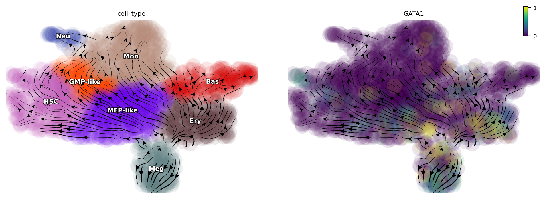
Mutual exclusive effects after perturbing either GATA1 or SPI1 gene
As we all know, GATA1 is the master regulator of the GMP lineage while SPI1 is the master regulator for the MEP lineage and GATA1 and PU1 forms a mutual inhibition and self-activation network motif.
We first suppress the expression of GATA1 and it can divert cells from GMP-related lineages to MEP-related lineages.
gene = "GATA1"
dyn.pd.perturbation(adata_labeling, gene, [-100], emb_basis="umap")
dyn.pl.streamline_plot(adata_labeling, color=["cell_type", gene], basis="umap_perturbation")
|-----> [projecting velocity vector to low dimensional embedding] in progress: 100.0000%
|-----> [projecting velocity vector to low dimensional embedding] finished [0.3502s]
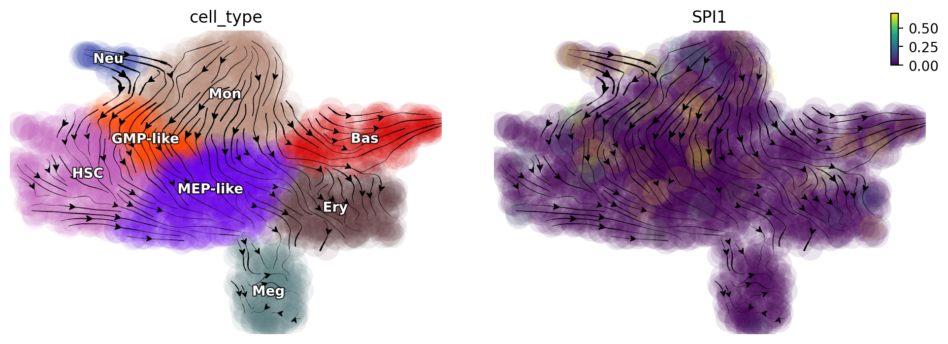
When suppressing the expression of SPI1, we find that cells from MEP-related lineages are diverted to GMP-related lineages.
gene = "SPI1"
dyn.pd.perturbation(adata_labeling, gene, [-100], emb_basis="umap")
dyn.pl.streamline_plot(adata_labeling, color=["cell_type", gene], basis="umap_perturbation")
|-----> [projecting velocity vector to low dimensional embedding] in progress: 100.0000%
|-----> [projecting velocity vector to low dimensional embedding] finished [0.3635s]
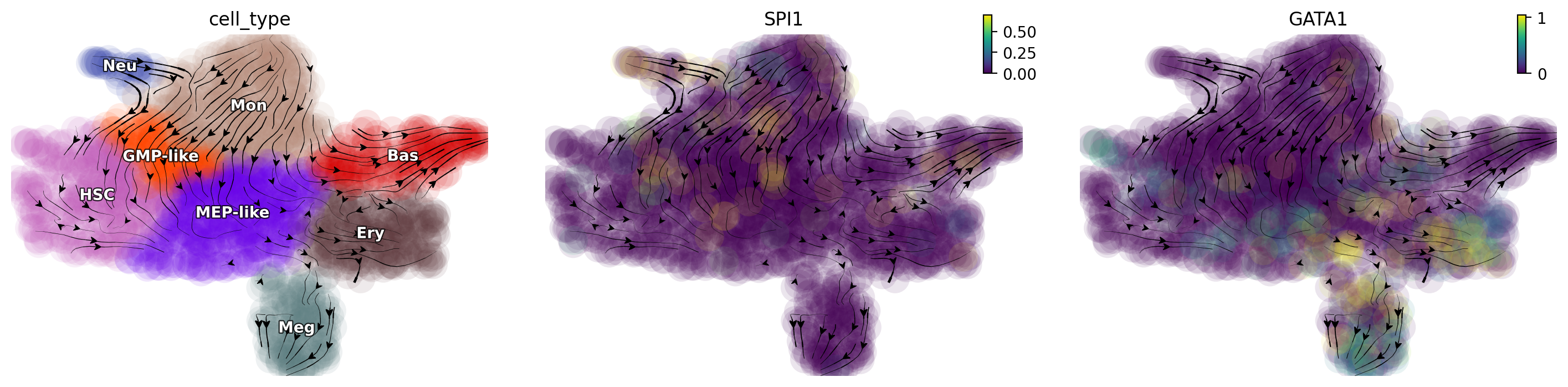
Double suppression of SPI1/GATA trap cell in the middle
Suppression of both SPI1 and GATA1 traps cells in the progenitor states. These predictions align well with those reported in (Rekhtman et al., 1999) and reveal a seesaw-effect regulation between SPI1 and GATA1 in driving the GMP and the MEP lineages.
selected_genes =  [ "SPI1", "GATA1"]
# expr_vals = [-100, -100]
expr_vals = [-100, -15]
dyn.pd.perturbation(adata_labeling, selected_genes, expr_vals, emb_basis="umap")
dyn.pl.streamline_plot(adata_labeling, color=["cell_type", gene], basis="umap_perturbation")
|-----> [projecting velocity vector to low dimensional embedding] in progress: 100.0000%
|-----> [projecting velocity vector to low dimensional embedding] finished [0.4156s]
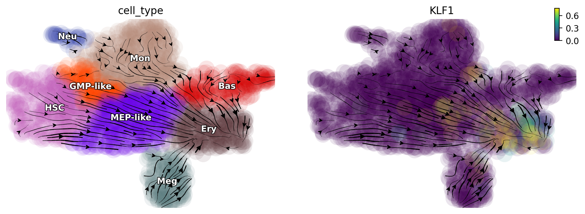
Activate KLF1
Dynamo in silico perturbation can correctly predicts other cellular transitions, showcased in [Qiu et al., 2022]. Here we show that activation of KLF1 leads other cells convert into erythroid cells, consistent with [Orkin and Zon, 2008].
gene = "KLF1"
dyn.pd.perturbation(adata_labeling, gene, [100], emb_basis="umap")
dyn.pl.streamline_plot(adata_labeling, color=["cell_type", gene], basis="umap_perturbation")
|-----> [projecting velocity vector to low dimensional embedding] in progress: 100.0000%
|-----> [projecting velocity vector to low dimensional embedding] finished [0.3362s]
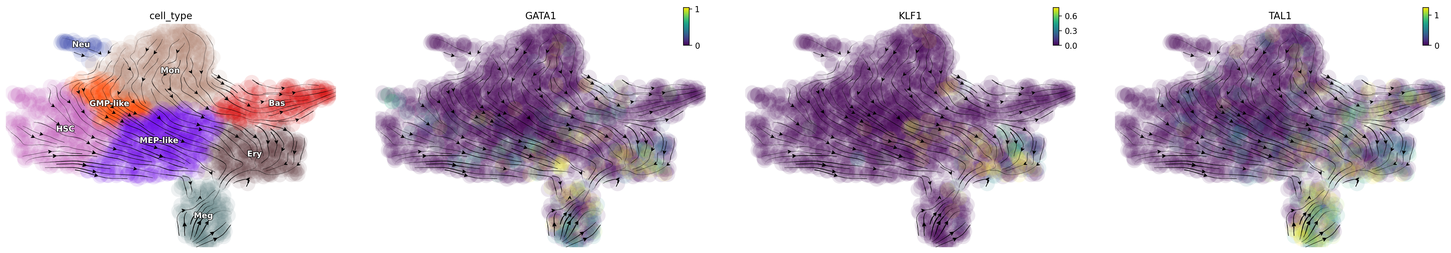
Triple activation of “GATA1”, “KLF1”, “TAL1”
Triple activation of GATA1, KLF1, and TAL1, known erythrocyte factors, and TFs used for reprogramming fibroblasts into erythrocytes, diverts most other cells into the Ery lineage [Capellera-Garcia et al., 2016].
selected_genes =  ["GATA1", "KLF1", "TAL1"]
expr_vals = [100, 100, 100]
dyn.pd.perturbation(adata_labeling, selected_genes, expr_vals, emb_basis="umap")
dyn.pl.streamline_plot(adata_labeling, color=["cell_type", gene], basis="umap_perturbation")
|-----> [projecting velocity vector to low dimensional embedding] in progress: 100.0000%
|-----> [projecting velocity vector to low dimensional embedding] finished [0.3842s]