

scNT-seq
This tutorial uses data from Qiu, Hu, et al (2020). Special thanks also go to Hao for the tutorial improvement.
In this study, by integrating metabolic RNA labeling, droplet microfluidics (Drop-seq) and chemical conversion of 4sU to cytosine analogs with TimeLapse chemistry, we developed scNT-seq to jointly profile newly-transcribed (marked by T-to-C substitutions) and pre-existing mRNAs from the same cell at scale. scNT-seq was used to distinguish new from old mRNAs using neuronal activity-induced genes in primary mouse cortical neurons. By linking cis-regulatory sequences to new transcripts, scNT-seq reveals time-resolved TF activity at single-cell levels.
We analyzed the scNT-seq with Dynamo to obtain time-resolved metabolic labeling based RNA velocity (computed from new and total RNA levels) which outperforms splicing RNA velocity (due to sparsity of intronic reads for many activity-induced genes) on inferring cell state trajectory during initial neuronal activation (0-30 min). Since dynamo explicitly models the labeling process and considers real time, the velocity learned is intrinsically physically meaningful (with the unit of molecules / hour).
Using pulse-chase labeling and scNT-seq, we further determined rates of RNA biogenesis and decay to uncover RNA regulatory strategies during stepwise conversion between pluripotent and rare totipotent two-cell embryo (2C)-like stem cell states.
Finally, we demonstrated that the library complexity can be substantially improved with 2nd strand synthesis reaction. This allows scNT-seq to detect ~6k genes and ~20k transcripts at ~50k reads per cell. We hope that this approach will be useful to many of you out there.
In this tutorial, we will use the newest dynamo to reanalyze the data and highlight a few analysis that is enabled with our vector field reconstruction algorithm. Please note that we recommend the reader to first go through our zerafish tutorial before diving into this tutorial.
# get the latest pypi version
# to get the latest version on github and other installations approaches, see:
# https://dynamo-release.readthedocs.io/en/latest/ten_minutes_to_dynamo.html#how-to-install
#!pip install dynamo-release --upgrade --quiet
import warnings
warnings.filterwarnings('ignore')
import dynamo as dyn
import numpy as np
import pandas as pd
import matplotlib.pyplot as plt
# dyn.get_all_dependencies_version()
Load splicing and labeling data
We prefiltered good quality cells for the labeling data. The same set of
high quality cells will also be used to subset the splicing data. We
especially focus on cells from excitatory neurons as they have the
strongest response to the KCL treatment.
neuron_labeling = dyn.sample_data.scNT_seq_neuron_labeling()
neuron_splicing = dyn.sample_data.scNT_seq_neuron_splicing()
|-----> Downloading data to ./data/neuron_labeling.h5ad
|-----> Downloading data to ./data/neuron_splicing.h5ad
print(neuron_labeling)
print(neuron_splicing)
AnnData object with n_obs × n_vars = 3060 × 24078
obs: 'cell_type', '4sU', 'treatment', 'time', 'cell_name'
var: 'gene_short_name', 'activity_genes'
layers: 'new', 'total'
AnnData object with n_obs × n_vars = 13476 × 44021
obs: 'cellname'
var: 'gene_short_name'
layers: 'spliced', 'unspliced'
Subset datasets with neural activity genes
Note that this labeling experiment is a mixture labeling experiment (See
discussion of labeling strategies
here).
In this experiment, the cells are all labeled for 2 hours (so we set
label_time as 2) but Kcl was added at different time point
prior to cell harvest. Therefore the neural cells will start from the
steady state, followed by an activation stage characterized by the
KCL-induced depolarization (except the 120 minutes time point).
Since the neural activation dynamics is intricate and happens on the
scale of 0-30 minutes, we need to focus our analysis on the subset of
neural activity genes (identified in Fig SI2d). Note that this
operation is specific for this system and generally not required for
systems with a longer time scale.
neuron_labeling.obs['label_time'] = 2 # this is the labeling time
tkey = 'label_time'
# Available at https://www.dropbox.com/s/h2rtmj3et098xba/0408_grp_info.txt?dl=0
# peng_gene_list = pd.read_csv('0408_grp_info.txt', sep='\t')
# neuron_labeling = neuron_labeling[:, peng_gene_list.index]
neuron_labeling = neuron_labeling[:, neuron_labeling.var.activity_genes]
Let us also subset the splicing data with the same set of cells and genes from the labeling data.
neuron_splicing = neuron_splicing[neuron_labeling.obs_names, neuron_labeling.var_names]
# neuron_labeling.obs['time'] = neuron_labeling.obs.time.astype('category')
neuron_labeling.obs['time'] = neuron_labeling.obs['time']/60
neuron_splicing.obs = neuron_labeling.obs.copy()
Run a typical dynamo analysis
This analysis consists the following five steps:
1. the preprocessing procedure;
2. kinetic estimation and velocity calculation;
3. dimension reduction;
4. high dimension velocity projection;
5. vector field reconstruction
Note that dynamo is smart enough to automatically detect your data type (splicing or labeling data) and choose the proper estimation method to analyze your data. The kinetic estimation and velocity calculation framework in dynamo is extremely sophisticated and comprehensive. See here for an overall description. Full details will be described in our final publication.
Note that setting calc_rnd_vel=True in dyn.tl.cell_velocities
will enable us to calculate randomized velocity which provides support
for the specificity of the observed time-resolved RNA velocity flow.
def dynamo_workflow(adata, **kwargs):
preprocessor = dyn.pp.Preprocessor(cell_cycle_score_enable=True)
preprocessor.preprocess_adata(adata, recipe='monocle', **kwargs)
# dyn.pp.recipe_monocle(adata, **kwargs)
dyn.tl.dynamics(adata)
dyn.tl.reduceDimension(adata)
dyn.tl.cell_velocities(adata, calc_rnd_vel=True, transition_genes=adata.var_names)
dyn.vf.VectorField(adata, basis='umap')
%%capture
dynamo_workflow(neuron_splicing)
dynamo_workflow(neuron_labeling, tkey='label_time', experiment_type='one-shot')
|-----> Running monocle preprocessing pipeline...
|-----------> filtered out 87 outlier cells
|-----------> filtered out 38 outlier genes
|-----> PCA dimension reduction
|-----> <insert> X_pca to obsm in AnnData Object.
|-----> computing cell phase...
|-----?
Dynamo is not able to perform cell cycle staging for you automatically.
Since dyn.pl.phase_diagram in dynamo by default colors cells by its cell-cycle stage,
you need to set color argument accordingly if confronting errors related to this.
|-----> dynamics_del_2nd_moments_key is None. Using default value from DynamoAdataConfig: dynamics_del_2nd_moments_key=False
|-----------> removing existing M layers:[]...
|-----------> making adata smooth...
|-----> <insert> X_umap to obsm in AnnData Object.
|-----> incomplete neighbor graph info detected: connectivities and distances do not exist in adata.obsp, indices not in adata.uns.neighbors.
|-----> Neighbor graph is broken, recomputing....
|-----? A new set of transition genes is used, but because enforce=False, the transition matrix might not be recalculated if it is found in .obsp.
|-----> 0 genes are removed because of nan velocity values.
|-----> [calculating transition matrix via pearson kernel with sqrt transform.] in progress: 100.0000%|-----> [calculating transition matrix via pearson kernel with sqrt transform.] completed [1.1513s]
|-----> [projecting velocity vector to low dimensional embedding] in progress: 100.0000%|-----> [projecting velocity vector to low dimensional embedding] completed [0.4293s]
|-----> [calculating transition matrix via pearson kernel with sqrt transform.] in progress: 100.0000%|-----> [calculating transition matrix via pearson kernel with sqrt transform.] completed [1.1340s]
|-----> [projecting velocity vector to low dimensional embedding] in progress: 100.0000%|-----> [projecting velocity vector to low dimensional embedding] completed [0.4278s]
|-----> Running monocle preprocessing pipeline...
|-----------> filtered out 0 outlier cells
|-----------> filtered out 0 outlier genes
|-----> PCA dimension reduction
|-----> <insert> X_pca to obsm in AnnData Object.
|-----> computing cell phase...
|-----?
Dynamo is not able to perform cell cycle staging for you automatically.
Since dyn.pl.phase_diagram in dynamo by default colors cells by its cell-cycle stage,
you need to set color argument accordingly if confronting errors related to this.
|-----> dynamics_del_2nd_moments_key is None. Using default value from DynamoAdataConfig: dynamics_del_2nd_moments_key=False
|-----------> removing existing M layers:[]...
|-----------> making adata smooth...
|-----? Your adata only has labeling data, but `NTR_vel` is set to be `False`. Dynamo will reset it to `True` to enable this analysis.
|-----> <insert> X_umap to obsm in AnnData Object.
|-----> incomplete neighbor graph info detected: connectivities and distances do not exist in adata.obsp, indices not in adata.uns.neighbors.
|-----> Neighbor graph is broken, recomputing....
|-----? A new set of transition genes is used, but because enforce=False, the transition matrix might not be recalculated if it is found in .obsp.
|-----> 0 genes are removed because of nan velocity values.
|-----> [calculating transition matrix via pearson kernel with sqrt transform.] in progress: 100.0000%|-----> [calculating transition matrix via pearson kernel with sqrt transform.] completed [1.2528s]
|-----> [projecting velocity vector to low dimensional embedding] in progress: 100.0000%|-----> [projecting velocity vector to low dimensional embedding] completed [0.4389s]
|-----> [calculating transition matrix via pearson kernel with sqrt transform.] in progress: 100.0000%|-----> [calculating transition matrix via pearson kernel with sqrt transform.] completed [1.2483s]
|-----> [projecting velocity vector to low dimensional embedding] in progress: 100.0000%|-----> [projecting velocity vector to low dimensional embedding] completed [0.4160s]
Time resolved dynamo velocity outperforms splicing velocity
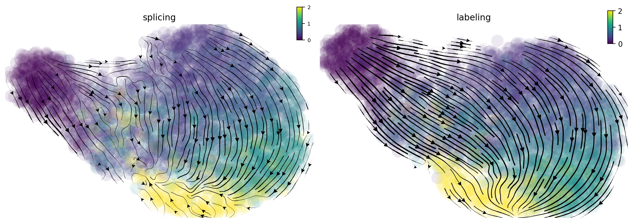
In the following, I will visualize the splicing (left) and labeling (right) velocity streamline plots side by side. Cells are color coded by time points. The streamlines indicate the integration paths that connect local projections from the observed state to the extrapolated future state. It is apparent that labeling velocity reveals a much more coherent trasition from cells at time 0 to 15, 30, 60 and 120 minutes than that of the splicing velocity. Interestingly, we can also see that the cells start with quick velocity until about 30 minutes and then slow down and gradually move backward to the original cell state at 120 minute, indicating a fast polorization phase followed a slow depolorization phase. Are those observed velocity results significant? Let us take a look at the randomized velocity results.
fig1, f1_axes = plt.subplots(ncols=2, nrows=1, constrained_layout=True, figsize=(12, 4))
f1_axes[0] = dyn.pl.streamline_plot(neuron_splicing, color='time', color_key_cmap = 'viridis', basis='umap', ax=f1_axes[0], show_legend='right', save_show_or_return='return')
f1_axes[0][0].set_title('splicing')
f1_axes[1] = dyn.pl.streamline_plot(neuron_labeling, color='time', color_key_cmap = 'viridis', basis='umap', ax=f1_axes[1], show_legend='right', save_show_or_return='return')
f1_axes[1][0].set_title('labeling')
plt.show()
|-----------> plotting with basis key=X_umap
|-----------> plotting with basis key=X_umap
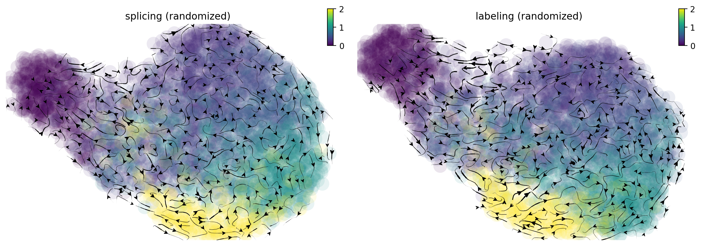
From the randomized velocity controls shown below for splicing kinetics or metabolic labeling-based RNA velocity, we can conclude our observed time-resolved RNA velocity is indeed highly specific and confident.
fig1, f1_axes = plt.subplots(ncols=2, nrows=1, constrained_layout=True, figsize=(12, 4))
f1_axes[0] = dyn.pl.streamline_plot(neuron_splicing, color='time', color_key_cmap = 'viridis', basis='umap_rnd', ax=f1_axes[0], show_legend='right', save_show_or_return='return')
f1_axes[0][0].set_title('splicing (randomized)')
f1_axes[1] = dyn.pl.streamline_plot(neuron_labeling, color='time', color_key_cmap = 'viridis', basis='umap_rnd', ax=f1_axes[1], show_legend='right', save_show_or_return='return')
f1_axes[1][0].set_title('labeling (randomized)')
plt.show()
|-----------> plotting with basis key=X_umap_rnd
|-----------> plotting with basis key=X_umap_rnd
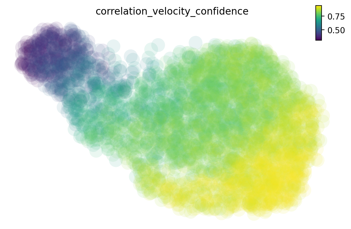
Calculate the cell-wise velocity confidence metric
There are many different methods to estimate the cell-wise velocity confidence. By default dynamo uses jaccard index, which measures how well each velocity vector meets the geometric constraints defined by the local neighborhood structure. Jaccard index is calculated as the fraction of the number of the intersected set of nearest neighbors from each cell at current expression state (X) and that from the future expression state (X + V) over the number of the union of these two sets. The cosine or correlation method is similar to that used by scVelo.
# you can also check the 'jaccord', 'cosine' or other methods
dyn.tl.cell_wise_confidence(neuron_labeling, ekey='M_t', vkey='velocity_T', method='correlation')
dyn.pl.umap(neuron_labeling, color='correlation_velocity_confidence')
calculating correlation based cell wise confidence: 100%|█| 3060/3060 [00:13<00:
|-----------> plotting with basis key=X_umap
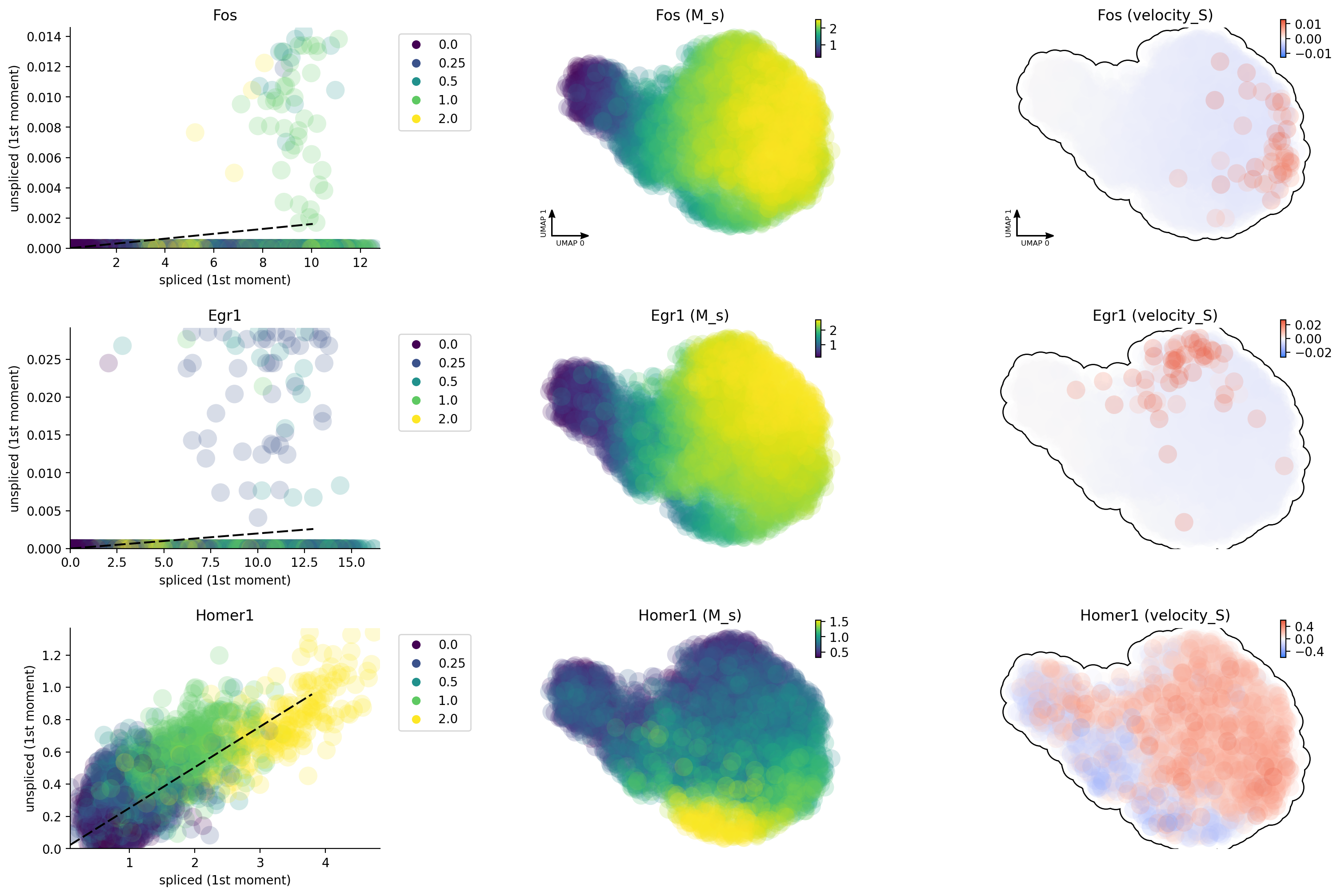
Why splicing velocity is worse?
One of the many reasons about why labeling based data is better than
conventional RNA velocity is that 4sU will label all nascent RNA in a
more uniform fashion while the capture of introns by mis-priming in
conventional scRNA-seq is highly biased due to sparsity of intronic
reads for many genes (especially those often lowly expressed
transcription factors or activity-induced genes as shown here). Here we
can see that, except Homer1, both Egr and Fos have very
insufficient intron reads, probably resulting from the lack of poly A/T
enriched regions in their introns.
gene_list = ["Egr1", "Fos", "Homer1"]
dyn.pl.phase_portraits(neuron_splicing, genes=gene_list, color='time', discrete_continous_div_color_key=[None, None, None], discrete_continous_div_color_key_cmap=['viridis', None, None], ncols=6, pointsize=5)
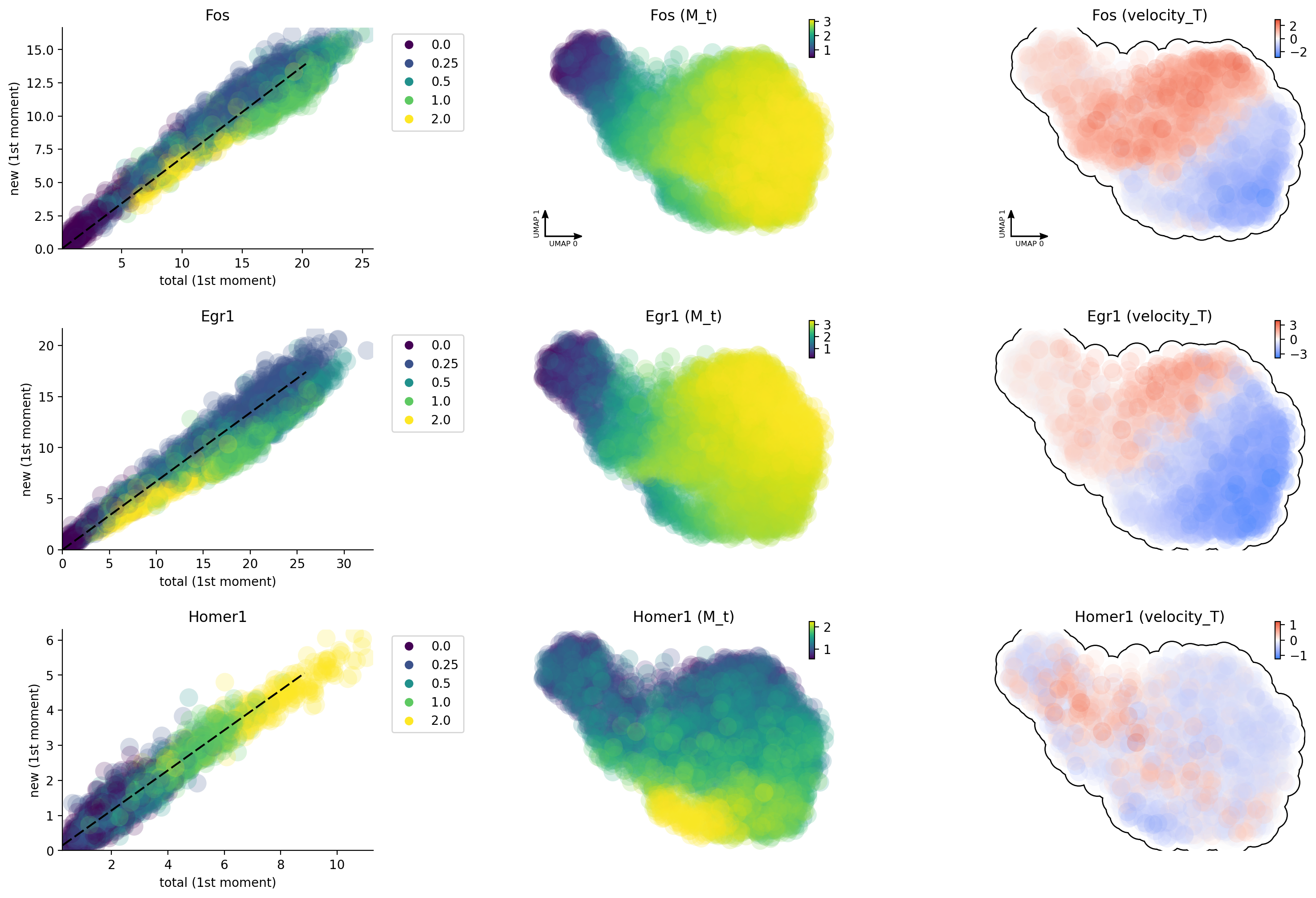
Unsprising, the labeling data gives us much improved capture of nascent RNA and reveals that Egr1 / Fos are early and immediate neural activation genes, respectively while Homer 1 is a late response gene. This is so cool!
dyn.pl.phase_portraits(neuron_labeling, genes=gene_list, color='time', discrete_continous_div_color_key=[None, None, None], discrete_continous_div_color_key_cmap=['viridis', None, None], ncols=6, pointsize=5)
Animate neural depolarization dynamics
In the following, let us also have some fun with animating neural activity response predictions via reconstructed vector field function
progenitor = neuron_labeling.obs_names[neuron_labeling.obs.time == 0]
np.random.seed(19491001)
from matplotlib import animation
info_genes = neuron_labeling.var_names[neuron_labeling.var.use_for_transition]
dyn.pd.fate(neuron_labeling, basis='umap', init_cells=progenitor, interpolation_num=100, direction='forward',
inverse_transform=False, average=False)
integration with ivp solver: 100%|████████████| 445/445 [00:15<00:00, 27.91it/s]
uniformly sampling points along a trajectory: 100%|█| 445/445 [00:00<00:00, 766.
AnnData object with n_obs × n_vars = 3060 × 97
obs: 'cell_type', '4sU', 'treatment', 'time', 'cell_name', 'label_time', 'nGenes', 'nCounts', 'pMito', 'pass_basic_filter', 'total_Size_Factor', 'initial_total_cell_size', 'new_Size_Factor', 'initial_new_cell_size', 'Size_Factor', 'initial_cell_size', 'ntr', 'control_point_umap', 'inlier_prob_umap', 'obs_vf_angle_umap', 'correlation_velocity_confidence'
var: 'gene_short_name', 'activity_genes', 'nCells', 'nCounts', 'pass_basic_filter', 'frac', 'use_for_pca', 'ntr', 'alpha', 'beta', 'gamma', 'half_life', 'alpha_b', 'alpha_r2', 'gamma_b', 'gamma_r2', 'gamma_logLL', 'delta_b', 'delta_r2', 'bs', 'bf', 'uu0', 'ul0', 'su0', 'sl0', 'U0', 'S0', 'total0', 'beta_k', 'gamma_k', 'use_for_dynamics', 'use_for_transition'
uns: 'pp', 'feature_selection', 'PCs', 'explained_variance_ratio_', 'pca_mean', 'dynamics', 'neighbors', 'umap_fit', 'grid_velocity_umap', 'grid_velocity_umap_rnd', 'VecFld_umap', 'fate_umap'
obsm: 'X_pca', 'X', 'X_umap', 'velocity_umap', 'X_umap_rnd', 'velocity_umap_rnd', 'velocity_umap_SparseVFC', 'X_umap_SparseVFC'
varm: 'alpha'
layers: 'new', 'total', 'X_total', 'X_new', 'M_t', 'M_tt', 'M_n', 'M_tn', 'M_nn', 'velocity_N', 'velocity_T'
obsp: 'moments_con', 'distances', 'connectivities', 'pearson_transition_matrix', 'pearson_transition_matrix_rnd'
%%capture
fig, ax = plt.subplots()
ax = dyn.pl.topography(neuron_labeling, color='time', ax=ax, save_show_or_return='return', color_key_cmap='viridis', figsize=(24, 24))
ax.set_aspect(0.8)
|-----------> plotting with basis key=X_umap
%%capture
neuron_labeling.obs['time'] = neuron_labeling.obs.time.astype('float')
instance = dyn.mv.StreamFuncAnim(adata=neuron_labeling, color='time', ax=ax)
|-----? the number of cell states with fate prediction is more than 50. You may want to lower the max number of cell states to draw via cell_states argument.
|-----------> plotting with basis key=X_umap
import matplotlib
matplotlib.rcParams['animation.embed_limit'] = 2**128 # Ensure all frames will be embedded.
from matplotlib import animation
import numpy as np
anim = animation.FuncAnimation(instance.fig, instance.update, init_func=instance.init_background,
frames=np.arange(100), interval=100, blit=True)
from IPython.core.display import display, HTML
HTML(anim.to_jshtml()) # embedding to jupyter notebook.