10 minutes to dynamo

Welcome to dynamo!

Dynamo is a computational framework that includes an inclusive model of expression dynamics with scSLAM-seq / multiomics, vector field reconstruction and potential landscape mapping.

Why dynamo

Dynamo currently provides a complete solution (see below) to analyze expression dynamics of conventional scRNA-seq or time-resolved metabolic labeling based scRNA-seq. It aspires to become the leading tools in continuously integrating the most exciting developments in machine learning, systems biology, information theory, stochastic physics, etc. to model, understand and interpret datasets generated from various cutting-edge single cell genomics techniques (developments of dynamo 2/3 is under way). We hope those models, understandings and interpretations not only facilitate your research but may also eventually lead to new biological discovery. Dynamo has a strong community so you will feel supported no matter you are a new-comer of computational biology or a veteran researcher who wants to contribute to dynamo’s development.

How to install

Dynamo requires Python 3.6 or later.

Dynamo now has been released to PyPi, you can install the PyPi version via:

pip install dynamo-release

To install the newest version of dynamo, you can git clone our repo and then pip install:

git clone https://github.com/aristoteleo/dynamo-release.git
pip install dynamo-release/ --user

Note that --user flag is used to install the package to your home directory, in case you don’t have the root privilege.

Alternatively, you can install dynamo when you are in the dynamo-release folder by directly using python’s setup install:

git clone https://github.com/aristoteleo/dynamo-release.git
cd dynamo-release/
python setup.py install --user

from source, using the following script:

pip install git+https://github.com:aristoteleo/dynamo-release

In order to ensure dynamo run properly, your python environment needs to satisfy dynamo’s dependencies. We provide a helper function for you to check the versions of dynamo’s all dependencies.

import dynamo as dyn
dyn.get_all_dependencies_version()

Architecture of dynamo

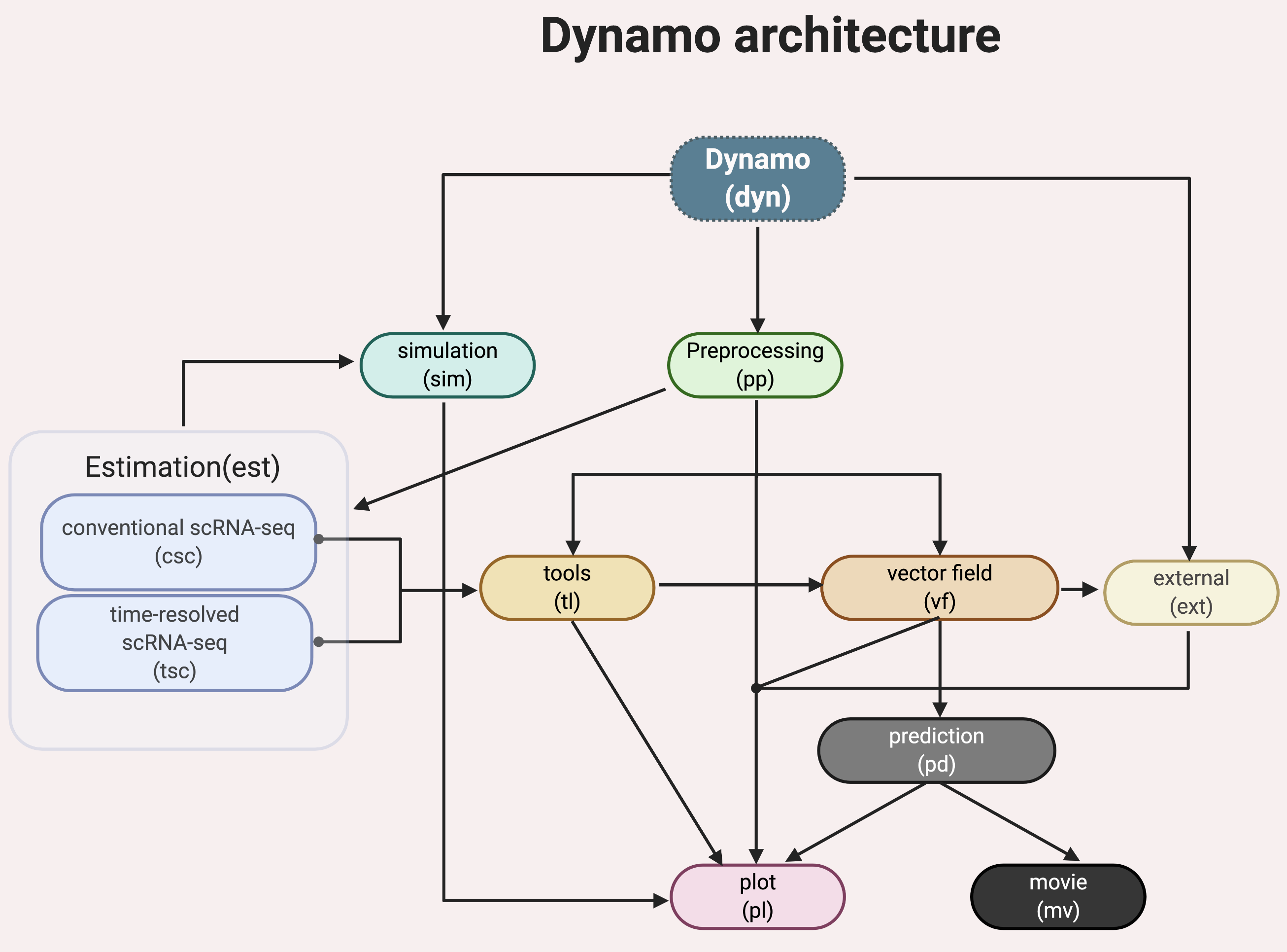
Dynamo has a few standard modules like most other single cell analysis toolkits (Scanpy, Monocle or Seurat), for example, data loading (dyn.read*), preprocessing (dyn.pp.*), tool analysis (dyn.tl.*), and plotting (dyn.pl.*). Modules specific to dynamo include:

• a comprehensive estimation framework (dyn.est.*) of expression dynamics that includes:

  • conventional single cell RNA-seq (scRNA-seq) modeling (dyn.est.csc.*) for standard RNA velocity estimation and more;

  • time-resolved metabolic labeling based single cell RNA-seq (scRNA-seq) modeling (dyn.est.tsc.*) for labeling based RNA velocity estimation and more;

• vector field reconstruction and vector calculus (dyn.vf.*);

• cell fate prediction (dyn.pd.*);

• create movie of cell fate predictions (dyn.mv.*);

• stochastic simulation of various metabolic labeling experiments (dyn.sim.*);

• integration with external tools built by us or others (dyn.ext.*);

• and more.

Typical workflow

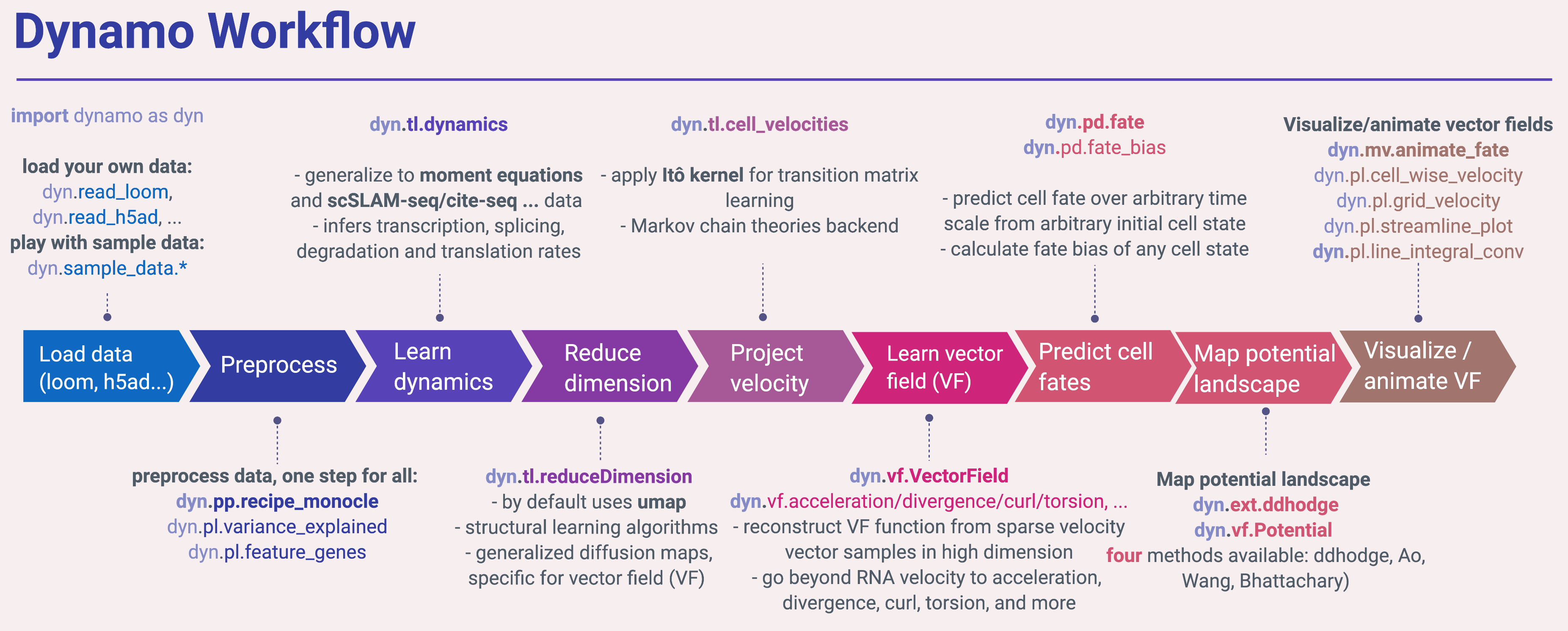
A typical workflow in dynamo is similar to most of other single cell analysis toolkits (Scanpy, Monocle or Seurat), including steps like importing dynamo (import dynamo as dyn), loading data (dyn.read*), preprocessing (dyn.pp.*), tool analysis (dyn.tl.*) and plotting (dyn.pl.*). To get the best of dynamo though, you need to use the dyn.vf.*, dyn.pd.* and dyn.mv.* modules.

Import dynamo as:

import dynamo as dyn

We provide a few nice visualization defaults for different purpose:

dyn.configuration.set_figure_params('dynamo', background='white') # jupter notebooks
dyn.configuration.set_figure_params('dynamo', background='black') # presentation
dyn.configuration.set_pub_style() # manuscript

Load data

Dynamo relies on anndata for data IO. You can read your own data via read, read_loom, read_h5ad, read_h5 or load_NASC_seq, etc:

adata = dyn.read(filename)

Dynamo also comes with a few builtin sample datasets so you can familiarize with dynamo before analyzing your own dataset. For example, you can load the Dentate Gyrus example dataset:

adata = dyn.sample_data.DentateGyrus()

There are many sample datasets available. You can check other available datasets via dyn.sample_data.*.

To process the scSLAM-seq data, please refer to the NASC-seq analysis pipeline. We are also working on a command line tool for this and will release it in due time. For processing splicing data, you can either use the velocyto command line interface or the bustool from Pachter lab.

Preprocess data

After loading data, you are ready to performs some preprocessing. You can run the recipe_monocle function that uses similar but generalized strategy from Monocle 3 to normalize all datasets in different layers (the spliced and unspliced or new, i.e. metabolic labelled, and total mRNAs or others), followed by feature selection and PCA dimension reduction.

dyn.pp.recipe_monocle(adata)

Learn dynamics

Next you will want to estimate the kinetic parameters of expression dynamics and then learn the velocity values for all genes that pass some filters (selected feature genes, by default) across cells. The dyn.tl.dynamics does all the hard work for you:

dyn.tl.dynamics(adata)

implicitly calls dyn.tl.moments first

dyn.tl.moments(adata)

which calculates the first, second moments (and sometimes covariance between different layers) of the expression data. First / second moments are basically mean and uncentered variance of gene expression, which are calculated based on local smoothing via a nearest neighbours graph, constructed in the reduced PCA space from the spliced or total mRNA expression of single cells.

And it then performs the following steps:

• checks the data you have and determine the experimental type automatically, either the conventional scRNA-seq, kinetics, degradation or one-shot single-cell metabolic labelling experiment or the CITE-seq or REAP-seq co-assay, etc.

• learns the velocity for each feature gene using either the original deterministic model based on a steady-state assumption from the seminal RNA velocity work or a few new methods, including the stochastic (default) or negative binomial method for conventional scRNA-seq or kinetic, degradation or one-shot models for metabolic labeling based scRNA-seq.

Those later methods are based on moment equations. All those methods use all or part of the output from dyn.tl.moments(adata).

Kinetic estimation of the conventional scRNA-seq and metabolic labeling based scRNA-seq is often tricky and has a lot pitfalls. Sometimes you may even observed undesired backward vector flow. You can evaluate the confidence of gene-wise velocity via:

dyn.tl.gene_wise_confidence(adata, group='group', lineage_dict={'Progenitor': ['terminal_cell_state']})

and filter those low confidence genes for downstream Velocity vectors analysis, etc (See more details in FAQ).

Dimension reduction

By default, we use umap algorithm for dimension reduction.

dyn.tl.reduceDimension(adata)

If the requested reduced dimension is already existed, dynamo won’t touch it unless you set enforce=True.

dyn.tl.reduceDimension(adata, basis='umap', enforce=True)

Velocity vectors

We need to project the velocity vector onto low dimensional embedding for later visualization. To get there, we can either use the default correlation/cosine kernel or the novel Itô kernel from us.

dyn.tl.cell_velocities(adata)

The above function projects and evaluates velocity vectors on umap space but you can also operate them on other basis, for example pca space:

dyn.tl.cell_velocities(adata, basis='pca')

You can check the confidence of cell-wise velocity to understand how reliable the recovered velocity is across cells via:

dyn.tl.cell_wise_confidence(adata)

Obviously dynamo doesn’t stop here. The really exciting part of dynamo lays in the fact that it learns a functional form of vector field in the full transcriptomic space which can be then used to predict cell fate and map single cell potential landscape.

Vector field reconstruction

In classical physics, including fluidics and aerodynamics, velocity and acceleration vector fields are used as fundamental tools to describe motion or external force of objects, respectively. In analogy, RNA velocity or protein accelerations estimated from single cells can be regarded as sparse samples in the velocity (La Manno et al. 2018) or acceleration vector field (Gorin, Svensson, and Pachter 2019) that defined on the gene expression space.

In general, a vector field can be defined as a vector-valued function f that maps any points (or cells’ expression state) x in a domain Ω with D dimension (or the gene expression system with D transcripts / proteins) to a vector y (for example, the velocity or acceleration for different genes or proteins), that is f(x) = y.

To formally define the problem of velocity vector field learning, we consider a set of measured cells with pairs of current and estimated future expression states. The difference between the predicted future state and current state for each cell corresponds to the velocity vector. We note that the measured single-cell velocity (conventional RNA velocity) is sampled from a smooth, differentiable vector field f that maps from xi to yi on the entire domain. Normally, single cell velocity measurements are results of biased, noisy and sparse sampling of the entire state space, thus the goal of velocity vector field reconstruction is to robustly learn a mapping function f that outputs yj given any point xj on the domain based on the observed data with certain smoothness constraints (Jiayi Ma et al. 2013). Under ideal scenario, the mapping function f should recover the true velocity vector field on the entire domain and predict the true dynamics in regions of expression space that are not sampled. To reconstruct vector field function in dynamo, you can simply use the following function to do all the heavy-lifting:

dyn.vf.VectorField(adata)

By default, it learns the vector field in the pca space but you can of course learn it in any space or even the original gene expression space.

Characterize vector field topology

Since we learn the vector field function of the data, we can then characterize the topology of the full vector field space. For example, we are able to identify

• the fixed points (attractor/saddles, etc.) which may corresponds to terminal cell types or progenitors;

• nullcline, separatrices of a recovered dynamic system, which may formally define the dynamical behaviour or the boundary of cell types in gene expression space.

Again, you only need to simply run the following function to get all those information.

dyn.vf.topography(adata, basis='umap')

Map potential landscape

The concept of potential landscape is widely appreciated across various biological disciplines, for example the adaptive landscape in population genetics, protein-folding funnel landscape in biochemistry, epigenetic landscape in developmental biology. In the context of cell fate transition, for example, differentiation, carcinogenesis, etc, a potential landscape will not only offers an intuitive description of the global dynamics of the biological process but also provides key insights to understand the multi-stability and transition rate between different cell types as well as to quantify the optimal path of cell fate transition.

Because the classical definition of potential function in physics requires gradient systems (no curl or cycling dynamics), which is often not applicable to open biological system. In dynamo we provided several ways to quantify the potential of single cells by decomposing the vector field into gradient, curl parts, etc. The recommended method is built on the Hodge decomposition on simplicial complexes (a sparse directional graph) constructed based on the learned vector field function that provides fruitful analogy of gradient, curl and harmonic (cyclic) flows on manifold:

dyn.ext.ddhodge(adata)

In addition, we and others proposed various strategies to decompose the stochastic differential equations into either the gradient or the curl component from first principles. We then can use the gradient part to define the potential.

Although an analytical decomposition on the reconstructed vector field is challenging, we are able to use a numerical algorithm we recently developed for our purpose. This approach uses a least action method under the A-type stochastic integration (Shi et al. 2012) to globally map the potential landscape Ψ(x) (Tang et al. 2017) by taking the vector field function f(x) as input.

dyn.vf.Potential(adata)

Visualization

In two or three dimensions, a streamline plot can be used to visualize the paths of cells will follow if released in different regions of the gene expression state space under a steady flow field. Although we currently do not support this, for vector field that changes over time, similar methods, for example, streakline, pathline, timeline, etc. can also be used to visualize the evolution of single cell or cell populations.

In dynamo, we have three standard visual representations of vector fields, including the cell wise, grid quiver plots and the streamline plot. Another intuitive way to visualize the structure of vector field is the so called line integral convolution method or LIC (Cabral and Leedom 1993), which works by adding random black-and-white paint sources on the vector field and letting the flowing particles on the vector field picking up some texture to ensure points on the same streamline having similar intensity. We relies on the yt’s annotate_line_integral_convolution function to visualize the LIC vector field reconstructed from dynamo.

dyn.pl.cell_wise_vectors(adata, color=colors, ncols=3)
dyn.pl.grid_vectors(adata, color=colors, ncols=3)
dyn.pl.stremline_plot(adata, color=colors, ncols=3)
dyn.pl.line_integral_conv(adata)

Note that colors here is a list or str that can be either the column name in .obs or gene names.

To visualize the topological structure of the reconstructed 2D vector fields, we provide the dyn.pl.topography function in dynamo.

dyn.vf.VectorField(adata, basis='umap')
dyn.pl.topography(adata)

Plotting functions in dynamo are designed to be extremely flexible. For example, you can combine different types of dynamo plots together (when you visualize only one item for each plot function)

import matplotlib.pyplot as plt
fig1, f1_axes = plt.subplots(ncols=2, nrows=2, constrained_layout=True, figsize=(12, 10))
f1_axes
f1_axes[0, 0] = dyn.pl.cell_wise_vectors(adata, color='umap_ddhodge_potential', pointsize=0.1, alpha = 0.7, ax=f1_axes[0, 0], quiver_length=6, quiver_size=6, save_show_or_return='return')
f1_axes[0, 1] = dyn.pl.grid_vectors(adata, color='speed_umap', ax=f1_axes[0, 1], quiver_length=12, quiver_size=12, save_show_or_return='return')
f1_axes[1, 0] = dyn.pl.streamline_plot(adata, color='divergence_pca', ax=f1_axes[1, 0], save_show_or_return='return')
f1_axes[1, 1] = dyn.pl.topography(adata, color='acceleration_umap', ax=f1_axes[1, 1], save_show_or_return='return')
plt.show()

The above creates a 2x2 plot that puts cell_wise_vectors, grid_vectors, streamline_plot and topography plots together.

Compatibility

Dynamo is fully compatible with velocyto, scanpy and scvelo. So you can use your loom or annadata object as input for dynamo. The velocity vector samples estimated from either velocyto or scvelo can be also directly used to reconstruct the functional form of vector field and to map the potential landscape in the entire expression space.