

Pancreatic endocrinogenesis differential geometry
In this tutorial, we will cover following topics:
learn contionus RNA velocity vector field functions in different spaces (e.g. umap or pca space)
rank genes based on the jacobian tensor
build and visualize gene regulatory network with top ranked genes
gene enrichment analyses of top ranked genes
visualize Jacobian derived regulatory interactions across cells
[1]:
# from IPython.core.display import display, HTML
# display(HTML("<style>.container { width:90% !important; }</style>"))
# %matplotlib inline
import warnings

warnings.filterwarnings("ignore")

import dynamo as dyn
|-----> setting visualization default mode in dynamo. Your customized matplotlib settings might be overritten.
Showing package dependecies which may help you debug dependency related bugs
[2]:
dyn.get_all_dependencies_version()
| package | dynamo-release | pre-commit | colorcet | cvxopt | loompy | matplotlib | networkx | numba | numdifftools | numpy | pandas | pynndescent | python-igraph | scikit-learn | scipy | seaborn | setuptools | statsmodels | tqdm | umap-learn |
|---|---|---|---|---|---|---|---|---|---|---|---|---|---|---|---|---|---|---|---|---|
| version | 1.0.0 | 2.16.0 | 2.0.6 | 1.2.7 | 3.0.6 | 3.4.3 | 2.6.3 | 0.54.1 | 0.9.40 | 1.20.3 | 1.3.4 | 0.5.5 | 0.9.8 | 1.0.2 | 1.8.0 | 0.11.2 | 58.0.4 | 0.13.2 | 4.62.3 | 0.5.2 |
Loading pancreatic endocrinogenesis dataset via dyn.sample_data
[3]:
dyn.configuration.set_figure_params("dynamo", background="white")
adata = dyn.sample_data.pancreatic_endocrinogenesis()
|-----> Downloading data to ./data/endocrinogenesis_day15.h5ad
|-----> [download] in progress: 100.0000%
|-----> [download] finished [5.4869s]
Defining pancreas_genes list, which we will investigate in the differential geometry analysis later in this notebook.
[4]:
pancreas_genes = [
    "Hes1",
    "Nkx6-1",
    "Nkx2-2",
    "Neurog3",
    "Neurod1",
    "Pax4",
    "Pax6",
    "Arx",
    "Pdx1",
    "Ins1",
    "Ins2",
    "Ghrl",
    "Ptf1a",
    "Iapp",
    "Isl1",
    "Sox9",
    "Gcg",
]
Proprocessing and learn RNA velocities
Normalizing adata with monocle recipe, reducing its dimension via PCA and computing velocities in PCA space
[5]:
dyn.pp.recipe_monocle(adata, n_top_genes=4000, fg_kwargs={"shared_count": 20}, genes_to_append=pancreas_genes)
dyn.tl.dynamics(adata, model="stochastic")
dyn.tl.reduceDimension(adata, n_pca_components=30)
dyn.tl.cell_velocities(adata, method="pearson", other_kernels_dict={"transform": "sqrt"})
dyn.tl.cell_velocities(adata, basis="pca")
|-----> recipe_monocle_keep_filtered_cells_key is None. Using default value from DynamoAdataConfig: recipe_monocle_keep_filtered_cells_key=True
|-----> recipe_monocle_keep_filtered_genes_key is None. Using default value from DynamoAdataConfig: recipe_monocle_keep_filtered_genes_key=True
|-----> recipe_monocle_keep_raw_layers_key is None. Using default value from DynamoAdataConfig: recipe_monocle_keep_raw_layers_key=True
|-----> apply Monocole recipe to adata...
|-----> <insert> pp to uns in AnnData Object.
|-----------> <insert> has_splicing to uns['pp'] in AnnData Object.
|-----------> <insert> has_labling to uns['pp'] in AnnData Object.
|-----------> <insert> splicing_labeling to uns['pp'] in AnnData Object.
|-----------> <insert> has_protein to uns['pp'] in AnnData Object.
|-----> ensure all cell and variable names unique.
|-----> ensure all data in different layers in csr sparse matrix format.
|-----> ensure all labeling data properly collapased
|-----------> <insert> tkey to uns['pp'] in AnnData Object.
|-----------> <insert> experiment_type to uns['pp'] in AnnData Object.
|-----> filtering cells...
|-----> <insert> pass_basic_filter to obs in AnnData Object.
|-----> 3696 cells passed basic filters.
|-----> filtering gene...
|-----> <insert> pass_basic_filter to var in AnnData Object.
|-----> 6956 genes passed basic filters.
|-----> calculating size factor...
|-----> selecting genes in layer: X, sort method: SVR...
|-----> <insert> frac to var in AnnData Object.
|-----> size factor normalizing the data, followed by log1p transformation.
|-----> Set <adata.X> to normalized data
|-----> applying PCA ...
|-----> <insert> pca_fit to uns in AnnData Object.
|-----> <insert> ntr to obs in AnnData Object.
|-----> <insert> ntr to var in AnnData Object.
|-----> cell cycle scoring...
|-----> computing cell phase...
|-----> [cell phase estimation] in progress: 100.0000%
|-----> [cell phase estimation] finished [11.3934s]
|-----> <insert> cell_cycle_phase to obs in AnnData Object.
|-----> <insert> cell_cycle_scores to obsm in AnnData Object.
|-----> [Cell Cycle Scores Estimation] in progress: 100.0000%
|-----> [Cell Cycle Scores Estimation] finished [0.2938s]
|-----> [recipe_monocle preprocess] in progress: 100.0000%
|-----> [recipe_monocle preprocess] finished [5.2262s]
|-----> dynamics_del_2nd_moments_key is None. Using default value from DynamoAdataConfig: dynamics_del_2nd_moments_key=False
|-----------> removing existing M layers:[]...
|-----------> making adata smooth...
|-----> calculating first/second moments...
OMP: Info #273: omp_set_nested routine deprecated, please use omp_set_max_active_levels instead.
|-----> [moments calculation] in progress: 100.0000%
|-----> [moments calculation] finished [17.8821s]
estimating gamma: 100%|██████████| 4000/4000 [02:28<00:00, 27.02it/s]
|-----> retrive data for non-linear dimension reduction...
|-----? adata already have basis umap. dimension reduction umap will be skipped!
set enforce=True to re-performing dimension reduction.
|-----> [dimension_reduction projection] in progress: 100.0000%
|-----> [dimension_reduction projection] finished [0.0007s]
|-----> 0 genes are removed because of nan velocity values.
|-----> [calculating transition matrix via pearson kernel with sqrt transform.] in progress: 100.0000%
|-----> [calculating transition matrix via pearson kernel with sqrt transform.] finished [4.4131s]
|-----> [projecting velocity vector to low dimensional embedding] in progress: 100.0000%
|-----> [projecting velocity vector to low dimensional embedding] finished [0.6581s]
|-----> 0 genes are removed because of nan velocity values.
Using existing pearson_transition_matrix found in .obsp.
|-----> [projecting velocity vector to low dimensional embedding] in progress: 100.0000%
|-----> [projecting velocity vector to low dimensional embedding] finished [0.7268s]
[5]:
AnnData object with n_obs × n_vars = 3696 × 27998
    obs: 'clusters_coarse', 'clusters', 'S_score', 'G2M_score', 'nGenes', 'nCounts', 'pMito', 'pass_basic_filter', 'Size_Factor', 'initial_cell_size', 'spliced_Size_Factor', 'initial_spliced_cell_size', 'unspliced_Size_Factor', 'initial_unspliced_cell_size', 'ntr', 'cell_cycle_phase'
    var: 'highly_variable_genes', 'nCells', 'nCounts', 'pass_basic_filter', 'log_m', 'log_cv', 'score', 'frac', 'use_for_pca', 'ntr', 'beta', 'gamma', 'half_life', 'alpha_b', 'alpha_r2', 'gamma_b', 'gamma_r2', 'gamma_logLL', 'delta_b', 'delta_r2', 'bs', 'bf', 'uu0', 'ul0', 'su0', 'sl0', 'U0', 'S0', 'total0', 'use_for_dynamics', 'use_for_transition'
    uns: 'clusters_coarse_colors', 'clusters_colors', 'day_colors', 'neighbors', 'pca', 'pp', 'velocyto_SVR', 'PCs', 'explained_variance_ratio_', 'pca_mean', 'pca_fit', 'feature_selection', 'cell_phase_genes', 'dynamics', 'grid_velocity_umap', 'grid_velocity_pca'
    obsm: 'X_pca', 'X_umap', 'X', 'cell_cycle_scores', 'velocity_umap', 'velocity_pca'
    layers: 'spliced', 'unspliced', 'X_spliced', 'X_unspliced', 'M_u', 'M_uu', 'M_s', 'M_us', 'M_ss', 'velocity_S'
    obsp: 'distances', 'connectivities', 'moments_con', 'pearson_transition_matrix'
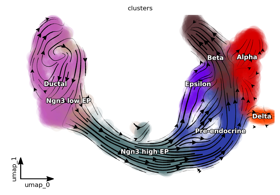
Visualize preprocessing results with a streamline plot on the umap basis.
[6]:
dyn.pl.streamline_plot(adata, color=["clusters"], basis="umap", show_legend="on data", show_arrowed_spines=True)
|-----------> plotting with basis key=X_umap
|-----------> skip filtering clusters by stack threshold when stacking color because it is not a numeric type
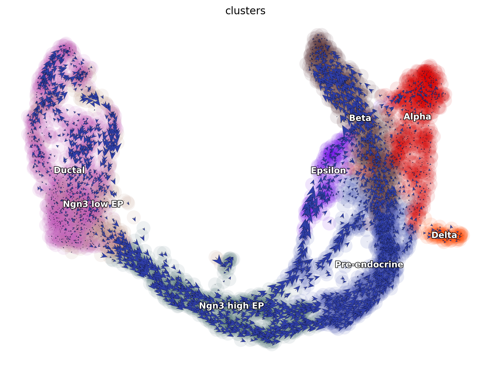
Visualizing cell velocity vectors via dyn.pl.cell_wise_vectors
[7]:
dyn.pl.cell_wise_vectors(
    adata,
    color=["clusters"],
    basis="umap",
    show_legend="on data",
    quiver_length=6,
    quiver_size=6,
    figsize=(8, 6),
    show_arrowed_spines=False,
)
|-----> X shape: (3696, 2) V shape: (3696, 2)
|-----------> plotting with basis key=X_umap
|-----------> skip filtering clusters by stack threshold when stacking color because it is not a numeric type
Differential geometry analyses reveal dynamics and key gene interactions
The diagram below illustrates the differentiation process of pancreatic endocrine cells and key regulatory genes/motifs.
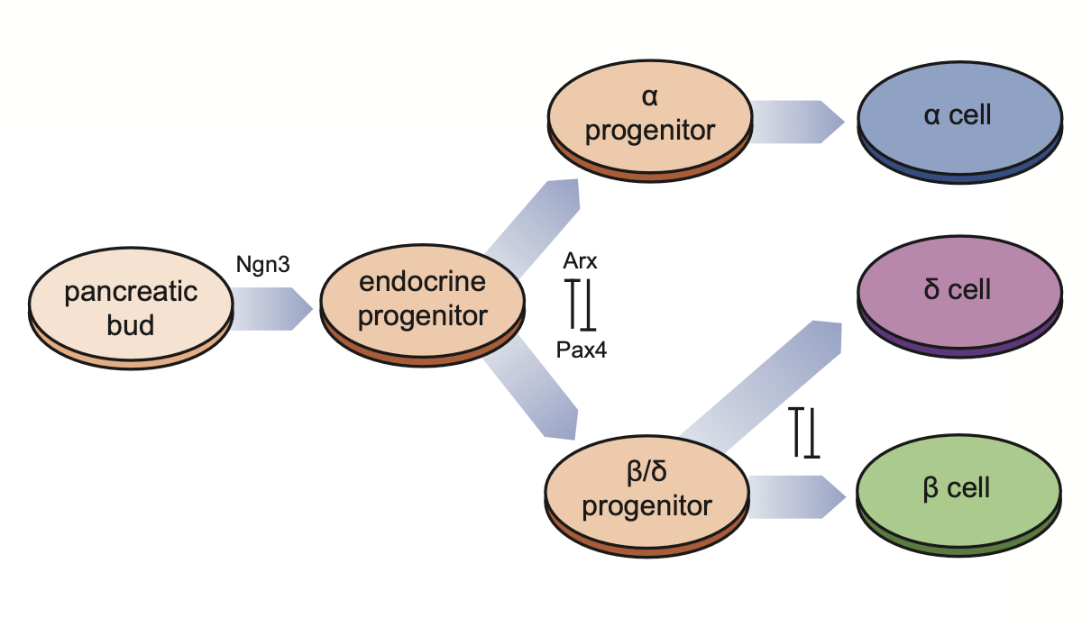
Define the progenitor cells: in this pancreatic endocrinogenesis dataset, we treat Doctal cells as progenitor cells.
[8]:
progenitor = adata.obs_names[adata.obs.clusters.isin(["Ductal"])]
len(progenitor)
[8]:
916
dynamo to learn a vectorfield. Here we learn the vectorfield on the pca basis. The vector field can be learned on the low dimensional embedding and can be then projected back to the high dimensional space.curl is defined in 2d/3d space, we use umap vectorfield to compute curl. umap and pca basis vectorfields will not interfere with each other (prefixed pca or umap) as you can check computation results in adata. You may try other embeddings such as PCA with fewer principe components to compute curl.Learning dynamics in PCA space via dyn.vf.VectorField and compute dynamics
[9]:
# dyn.tl.cell_velocities(adata, basis="pca")
dyn.vf.VectorField(adata, basis="pca", pot_curl_div=True)
dyn.vf.VectorField(adata, basis="umap", pot_curl_div=True)

dyn.vf.speed(adata, basis="pca")
dyn.vf.divergence(adata, basis="pca")
dyn.vf.acceleration(adata, basis="pca")
dyn.vf.curl(adata, basis="umap")
|-----> VectorField reconstruction begins...
|-----> Retrieve X and V based on basis: PCA.
        Vector field will be learned in the PCA space.
|-----> Learning vector field with method: sparsevfc.
|-----> [SparseVFC] begins...
|-----> Sampling control points based on data velocity magnitude...
|-----> [SparseVFC] in progress: 100.0000%
|-----> [SparseVFC] finished [0.3509s]
|-----> <insert> velocity_pca_SparseVFC to obsm in AnnData Object.
|-----> <insert> X_pca_SparseVFC to obsm in AnnData Object.
|-----> <insert> VecFld_pca to uns in AnnData Object.
|-----> Running ddhodge to estimate vector field based pseudotime in pca basis...
|-----> graphizing vectorfield...
|-----> incomplete neighbor graph info detected: connectivities and distances do not exist in adata.obsp, indices not in adata.uns.neighbors.
|-----> Neighbor graph is broken, recomputing....
|-----> Start computing neighbor graph...
|-----------> X_data is None, fetching or recomputing...
|-----> fetching X data from layer:None, basis:pca
|-----> method arg is None, choosing methods automatically...
|-----------> method ball_tree selected
|-----> <insert> connectivities to obsp in AnnData Object.
|-----> <insert> distances to obsp in AnnData Object.
|-----> <insert> neighbors to uns in AnnData Object.
|-----> <insert> neighbors.indices to uns in AnnData Object.
|-----> <insert> neighbors.params to uns in AnnData Object.
|-----------? nbrs_idx argument is ignored and recomputed because nbrs_idx is not None and return_nbrs=True
|-----------> calculating neighbor indices...
|-----> [ddhodge completed] in progress: 100.0000%
|-----> [ddhodge completed] finished [19.4571s]
|-----> Computing divergence...
Calculating divergence: 100%|██████████| 4/4 [00:00<00:00, 11.73it/s]
|-----> <insert> control_point_pca to obs in AnnData Object.
|-----> <insert> inlier_prob_pca to obs in AnnData Object.
|-----> <insert> obs_vf_angle_pca to obs in AnnData Object.
|-----> [VectorField] in progress: 100.0000%
|-----> [VectorField] finished [20.2223s]
|-----> VectorField reconstruction begins...
|-----> Retrieve X and V based on basis: UMAP.
        Vector field will be learned in the UMAP space.
|-----> Generating high dimensional grids and convert into a row matrix.
|-----> Learning vector field with method: sparsevfc.
|-----> [SparseVFC] begins...
|-----> Sampling control points based on data velocity magnitude...
|-----> [SparseVFC] in progress: 100.0000%
|-----> [SparseVFC] finished [0.9759s]
|-----> <insert> velocity_umap_SparseVFC to obsm in AnnData Object.
|-----> <insert> X_umap_SparseVFC to obsm in AnnData Object.
|-----> <insert> VecFld_umap to uns in AnnData Object.
|-----> Running ddhodge to estimate vector field based pseudotime in umap basis...
|-----> graphizing vectorfield...
|-----------? nbrs_idx argument is ignored and recomputed because nbrs_idx is not None and return_nbrs=True
|-----------> calculating neighbor indices...
|-----> [ddhodge completed] in progress: 100.0000%
|-----> [ddhodge completed] finished [20.8427s]
|-----> Computing curl...
Calculating 2-D curl: 100%|██████████| 3696/3696 [00:00<00:00, 27838.20it/s]
|-----> Computing divergence...
Calculating divergence: 100%|██████████| 4/4 [00:00<00:00, 33.65it/s]
|-----> <insert> control_point_umap to obs in AnnData Object.
|-----> <insert> inlier_prob_umap to obs in AnnData Object.
|-----> <insert> obs_vf_angle_umap to obs in AnnData Object.
|-----> [VectorField] in progress: 100.0000%
|-----> [VectorField] finished [22.1098s]
Calculating divergence: 100%|██████████| 4/4 [00:00<00:00, 11.50it/s]
|-----> [Calculating acceleration] in progress: 100.0000%
|-----> [Calculating acceleration] finished [0.1408s]
|-----> <insert> acceleration to layers in AnnData Object.
Calculating 2-D curl: 100%|██████████| 3696/3696 [00:00<00:00, 28036.52it/s]
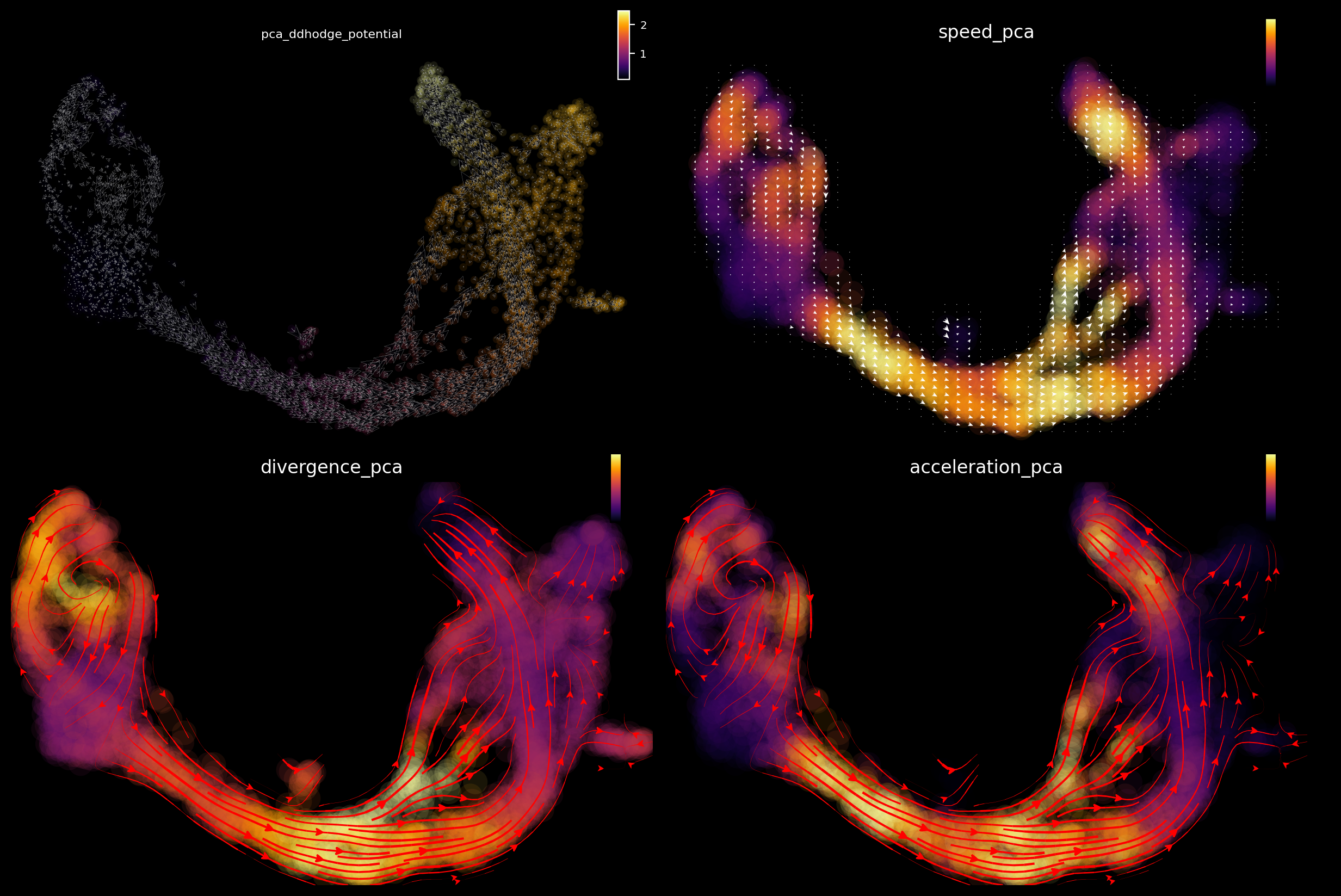
The acceleration and divergence accurately highlight hotspots, including a saddle point in ductal cells (negative divergence), exit from this state to early endocrine progenitors (high positive acceleration), the bifurcation point for late progenitors to differentiate into stable cell types (high acceleration and positive divergence), and stable cell types (negative divergence).
[10]:
dyn.configuration.set_figure_params("dynamo", background="black")

import matplotlib.pyplot as plt

fig1, fig1_axes = plt.subplots(ncols=2, nrows=2, constrained_layout=True, figsize=(12, 8))
dyn.pl.cell_wise_vectors(
    adata,
    color="pca_ddhodge_potential",
    pointsize=0.1,
    alpha=0.7,
    ax=fig1_axes[0, 0],
    quiver_length=6,
    quiver_size=6,
    save_show_or_return="return",
    background="black",
)
dyn.pl.grid_vectors(
    adata,
    color="speed_pca",
    basis="umap",
    ax=fig1_axes[0, 1],
    quiver_length=12,
    quiver_size=12,
    save_show_or_return="return",
    background="black",
)
dyn.pl.streamline_plot(
    adata, color="divergence_pca", basis="umap", ax=fig1_axes[1, 0], save_show_or_return="return", background="black"
)
dyn.pl.streamline_plot(
    adata, color="acceleration_pca", basis="umap", ax=fig1_axes[1, 1], save_show_or_return="return", background="black"
)
plt.show()
|-----> X shape: (3696, 2) V shape: (3696, 2)
|-----------> plotting with basis key=X_umap
|-----------> plotting with basis key=X_umap
|-----------> plotting with basis key=X_umap
|-----------> plotting with basis key=X_umap
Visualizing vectorfield attractors and saddle points via dyn.pl.topography
The following 2D UMAP vector field topology shows stable fixed points (attractors) in alpha, beta, and ductal cells, and a saddle point #6 at the branching point between ductal cells and early progenitors.
[11]:
dyn.pl.topography(
    adata, basis="umap", background="white", color=["clusters"], streamline_color="black", show_legend="on data"
)
|-----> Vector field for umap is but its topography is not mapped. Mapping topography now ...
|-----------> plotting with basis key=X_umap
|-----------> skip filtering clusters by stack threshold when stacking color because it is not a numeric type
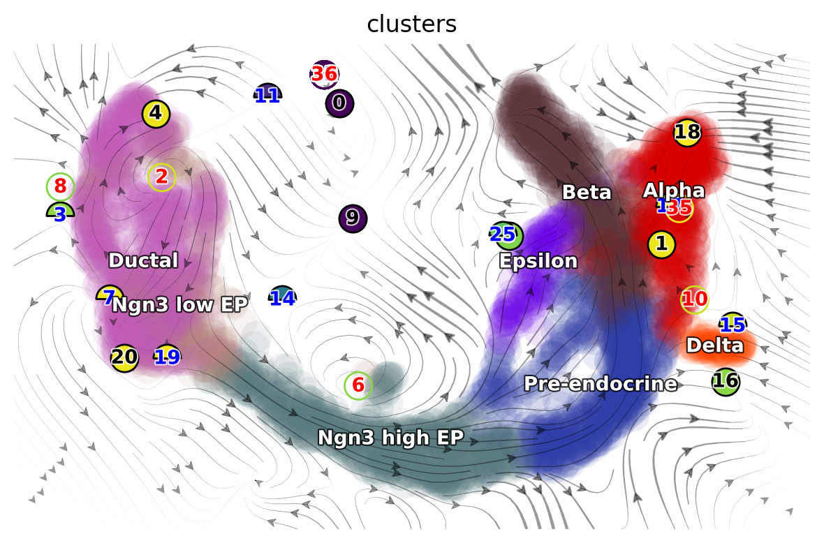
From the results above, we can observe that high acceleration is observed at the interface between early and late progenitors (magnitude change in velocity), and the bifurcation point where progenitors differentiate into stable cell types (direction change in velocity). Negative divergence is observed at the saddle point and attractors, and positive divergence at the bifurcation point and cell cycle of pancreatic buds.
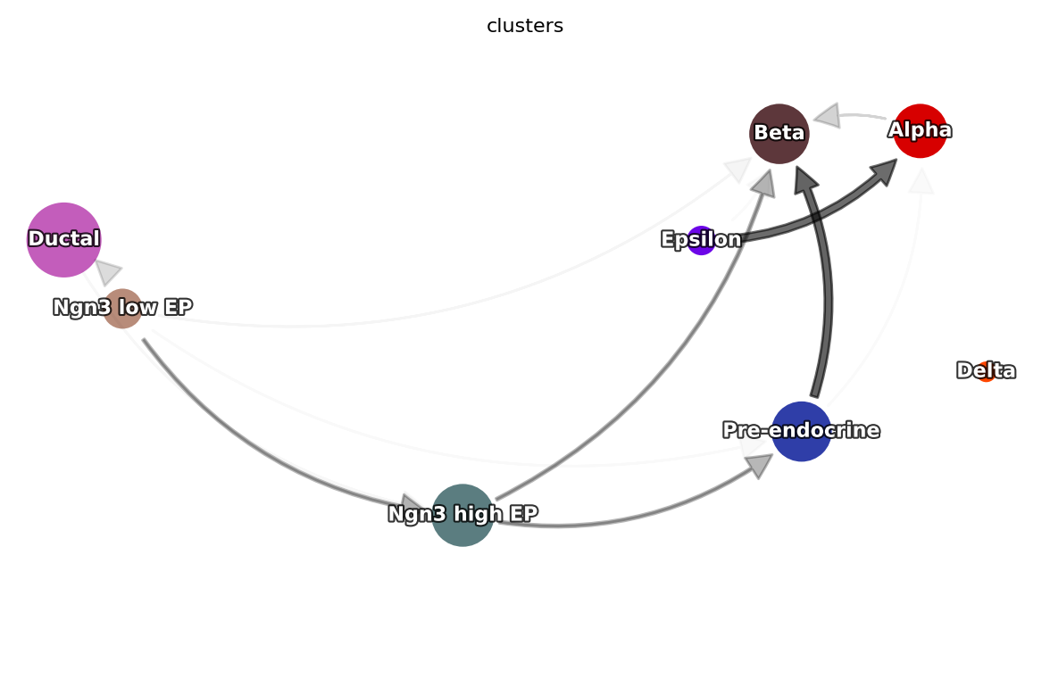
Constructing a cell type state transition graph
[12]:
dyn.configuration.set_figure_params("dynamo", background="white")
dyn.pd.state_graph(adata, group='clusters', basis='pca', method='vf')
dyn.pl.state_graph(adata,
                   color=['clusters'],
                   group='clusters',
                   basis='umap',
                   show_legend='on data',
                   method='vf');
|-----> Estimating the transition probability between cell types...
|-----> Applying vector field
|-----> [KDTree computation] in progress: 100.0000%in progress: 0.0000%
|-----> [KDTree computation] finished [0.0013s]
|-----> [iterate groups] in progress: 12.5000%
integration with ivp solver: 100%|██████████| 100/100 [00:03<00:00, 25.14it/s]
uniformly sampling points along a trajectory: 100%|██████████| 100/100 [00:00<00:00, 146.29it/s]
|-----> [iterate groups] in progress: 25.0000%
integration with ivp solver: 100%|██████████| 100/100 [00:04<00:00, 22.93it/s]
uniformly sampling points along a trajectory: 100%|██████████| 100/100 [00:00<00:00, 144.02it/s]
|-----> [iterate groups] in progress: 37.5000%
integration with ivp solver: 100%|██████████| 100/100 [00:04<00:00, 24.49it/s]
uniformly sampling points along a trajectory: 100%|██████████| 100/100 [00:00<00:00, 142.90it/s]
|-----> [iterate groups] in progress: 50.0000%
integration with ivp solver: 100%|██████████| 100/100 [00:04<00:00, 22.77it/s]
uniformly sampling points along a trajectory: 100%|██████████| 100/100 [00:00<00:00, 135.77it/s]
|-----> [iterate groups] in progress: 62.5000%
integration with ivp solver: 100%|██████████| 70/70 [00:02<00:00, 31.55it/s]
uniformly sampling points along a trajectory: 100%|██████████| 70/70 [00:00<00:00, 144.03it/s]
|-----> [iterate groups] in progress: 75.0000%
integration with ivp solver: 100%|██████████| 100/100 [00:03<00:00, 26.10it/s]
uniformly sampling points along a trajectory: 100%|██████████| 100/100 [00:00<00:00, 139.76it/s]
|-----> [iterate groups] in progress: 87.5000%
integration with ivp solver: 100%|██████████| 100/100 [00:04<00:00, 23.40it/s]
uniformly sampling points along a trajectory: 100%|██████████| 100/100 [00:00<00:00, 146.82it/s]
|-----> [iterate groups] in progress: 100.0000%
integration with ivp solver: 100%|██████████| 100/100 [00:04<00:00, 24.71it/s]
uniformly sampling points along a trajectory: 100%|██████████| 100/100 [00:00<00:00, 137.70it/s]
|-----> [iterate groups] in progress: 100.0000%
|-----> [iterate groups] finished [42.2887s]
|-----> [State graph estimation] in progress: 100.0000%
|-----> [State graph estimation] finished [0.0012s]
|-----------> plotting with basis key=X_umap
|-----------> skip filtering clusters by stack threshold when stacking color because it is not a numeric type
<Figure size 600x400 with 0 Axes>
Computing Jacobian and reveal regulator/effector gene relations via dyn.vf.jacobian
[13]:
dyn.vf.jacobian(adata, regulators=pancreas_genes)
Transforming subset Jacobian: 100%|██████████| 3696/3696 [00:00<00:00, 59324.06it/s]
[13]:
AnnData object with n_obs × n_vars = 3696 × 27998
    obs: 'clusters_coarse', 'clusters', 'S_score', 'G2M_score', 'nGenes', 'nCounts', 'pMito', 'pass_basic_filter', 'Size_Factor', 'initial_cell_size', 'spliced_Size_Factor', 'initial_spliced_cell_size', 'unspliced_Size_Factor', 'initial_unspliced_cell_size', 'ntr', 'cell_cycle_phase', 'pca_ddhodge_div', 'pca_ddhodge_potential', 'divergence_pca', 'control_point_pca', 'inlier_prob_pca', 'obs_vf_angle_pca', 'umap_ddhodge_div', 'umap_ddhodge_potential', 'curl_umap', 'divergence_umap', 'control_point_umap', 'inlier_prob_umap', 'obs_vf_angle_umap', 'speed_pca', 'acceleration_pca', 'jacobian_det_pca'
    var: 'highly_variable_genes', 'nCells', 'nCounts', 'pass_basic_filter', 'log_m', 'log_cv', 'score', 'frac', 'use_for_pca', 'ntr', 'beta', 'gamma', 'half_life', 'alpha_b', 'alpha_r2', 'gamma_b', 'gamma_r2', 'gamma_logLL', 'delta_b', 'delta_r2', 'bs', 'bf', 'uu0', 'ul0', 'su0', 'sl0', 'U0', 'S0', 'total0', 'use_for_dynamics', 'use_for_transition'
    uns: 'clusters_coarse_colors', 'clusters_colors', 'day_colors', 'neighbors', 'pca', 'pp', 'velocyto_SVR', 'PCs', 'explained_variance_ratio_', 'pca_mean', 'pca_fit', 'feature_selection', 'cell_phase_genes', 'dynamics', 'grid_velocity_umap', 'grid_velocity_pca', 'VecFld_pca', 'VecFld_umap', 'clusters_graph', 'jacobian_pca'
    obsm: 'X_pca', 'X_umap', 'X', 'cell_cycle_scores', 'velocity_umap', 'velocity_pca', 'velocity_pca_SparseVFC', 'X_pca_SparseVFC', 'velocity_umap_SparseVFC', 'X_umap_SparseVFC', 'acceleration_pca'
    layers: 'spliced', 'unspliced', 'X_spliced', 'X_unspliced', 'M_u', 'M_uu', 'M_s', 'M_us', 'M_ss', 'velocity_S', 'acceleration'
    obsp: 'distances', 'connectivities', 'moments_con', 'pearson_transition_matrix', 'pca_ddhodge', 'umap_ddhodge'
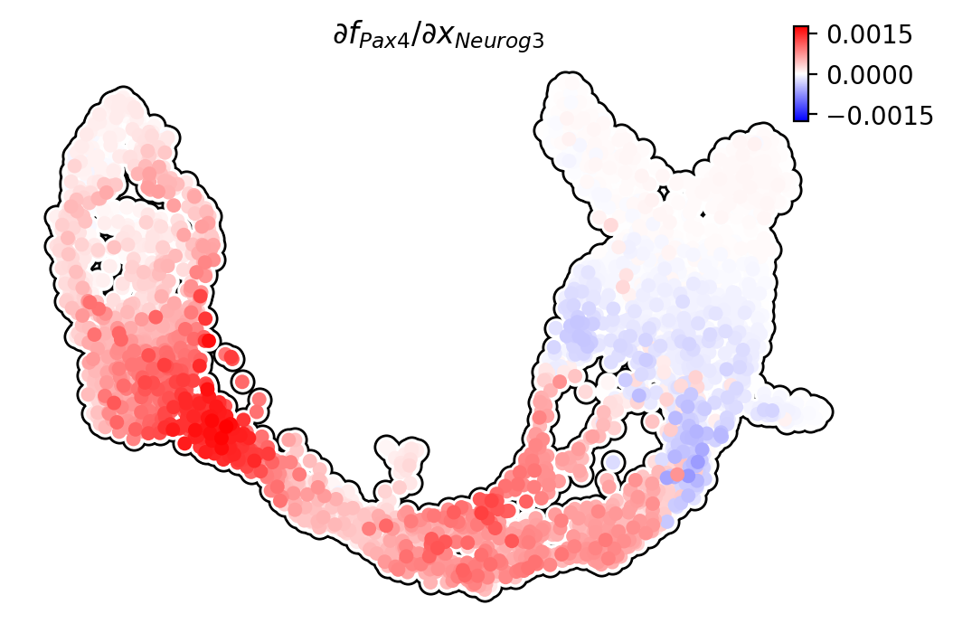
Pax4/Neurog3
Ngn3 activates Pax4 in progenitors, initiating pancreatic endocrinogenesis
[14]:
dyn.pl.jacobian(
    adata,
    basis="umap",
    regulators=[
        "Neurog3",
    ],
    effectors=["Pax4"],
    alpha=1,
)
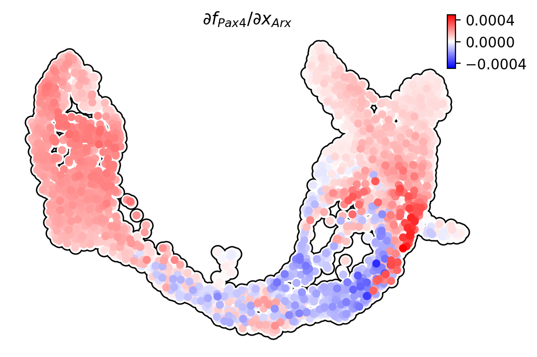
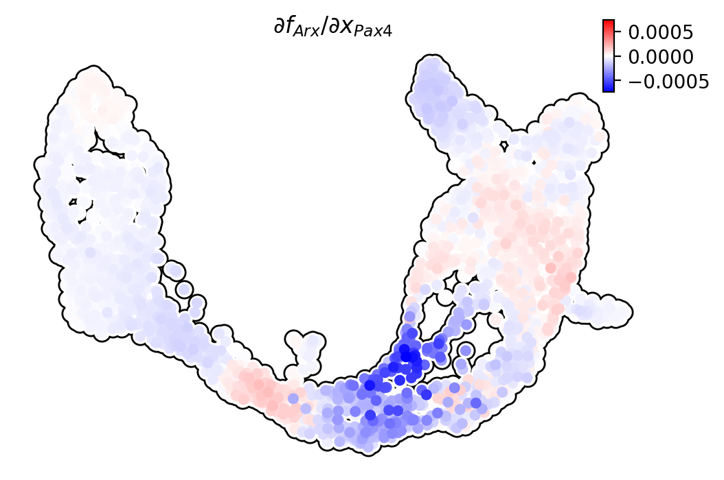
Pax4/Arx
Jacobian analyses reveal mutual inhibition of Pax4 and Arx at the bifurcation point in progenitors.
[15]:
dyn.pl.jacobian(adata, basis="umap", regulators=["Arx"], effectors=["Pax4"], alpha=1)
[16]:
dyn.pl.jacobian(adata, basis="umap", regulators=["Pax4"], effectors=["Arx"], alpha=1)
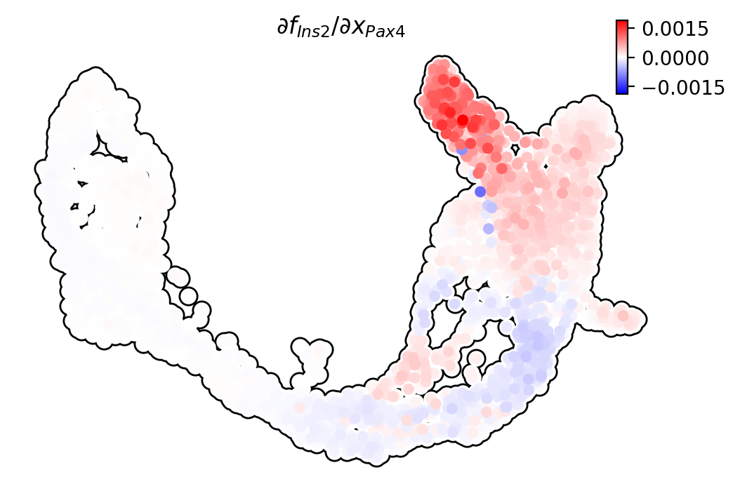
Pax4/Ins2
Pdx1 activates Ins2 in beta cells.
[17]:
dyn.pl.jacobian(adata, basis="umap", regulators=["Pax4"], effectors=["Ins2"], alpha=1)
[18]:
adata.obs["clusters"].unique()
[18]:
['Pre-endocrine', 'Ductal', 'Alpha', 'Ngn3 high EP', 'Delta', 'Beta', 'Ngn3 low EP', 'Epsilon']
Categories (8, object): ['Ductal', 'Ngn3 low EP', 'Ngn3 high EP', 'Pre-endocrine', 'Beta', 'Alpha', 'Delta', 'Epsilon']
We can rank the elements in the Jacobian. There are 5 ways to rank the Jacobian:
'full_reg': top regulators are ranked for each effector for each cell group;'full_eff': top effectors are ranked for each regulator for each cell group;‘
reg’: top regulators in each cell group;‘
eff’: top effectors in each cell group;‘
int’: top effector-regulator pairs in each cell group.
The default mdoe is 'full_reg'. Note that in full_reg and full_eff modes, a dictionary mapping clusters (cell type) to ranking dataframes is returned by dyn.vf.rank_jacobian_genes.
[19]:
full_reg_rank = dyn.vf.rank_jacobian_genes(
    adata, groups="clusters", mode="full_reg", abs=True, output_values=True, return_df=True
)
full_eff_rank = dyn.vf.rank_jacobian_genes(
    adata, groups="clusters", mode="full_eff", abs=True, exclude_diagonal=True, output_values=True, return_df=True
)
[20]:
full_reg_rank['Pre-endocrine'][:5]
[20]:
| Neurog3 | Neurog3_values | Sox9 | Sox9_values | Isl1 | Isl1_values | Hes1 | Hes1_values | Ins1 | Ins1_values | Gcg | Gcg_values | Neurod1 | Neurod1_values | Nkx2-2 | Nkx2-2_values | Ptf1a | Ptf1a_values | Pax6 | Pax6_values | Nkx6-1 | Nkx6-1_values | Pdx1 | Pdx1_values | Pax4 | Pax4_values | Ghrl | Ghrl_values | Iapp | Iapp_values | Ins2 | Ins2_values | Arx | Arx_values | |
|---|---|---|---|---|---|---|---|---|---|---|---|---|---|---|---|---|---|---|---|---|---|---|---|---|---|---|---|---|---|---|---|---|---|---|
| 0 | Neurog3 | 0.000569 | Gcg | 0.000232 | Gcg | 0.000681 | Gcg | 0.000089 | Gcg | 0.000504 | Gcg | 0.001130 | Neurog3 | 0.000081 | Ghrl | 0.000043 | Gcg | 0.000019 | Gcg | 0.000283 | Isl1 | 0.000492 | Isl1 | 0.000357 | Neurog3 | 0.000335 | Ghrl | 0.002203 | Iapp | 0.001547 | Gcg | 0.000455 | Isl1 | 0.000319 |
| 1 | Iapp | 0.000453 | Iapp | 0.000186 | Isl1 | 0.000663 | Iapp | 0.000076 | Iapp | 0.000396 | Ghrl | 0.000568 | Iapp | 0.000070 | Iapp | 0.000032 | Ghrl | 0.000016 | Isl1 | 0.000251 | Ghrl | 0.000390 | Pdx1 | 0.000329 | Isl1 | 0.000251 | Isl1 | 0.000795 | Isl1 | 0.001015 | Isl1 | 0.000356 | Arx | 0.000288 |
| 2 | Gcg | 0.000402 | Neurog3 | 0.000115 | Nkx6-1 | 0.000399 | Isl1 | 0.000063 | Ins1 | 0.000365 | Isl1 | 0.000251 | Isl1 | 0.000062 | Isl1 | 0.000026 | Iapp | 0.000015 | Neurog3 | 0.000224 | Neurog3 | 0.000370 | Arx | 0.000306 | Iapp | 0.000233 | Pax4 | 0.000493 | Gcg | 0.000834 | Ins1 | 0.000354 | Pdx1 | 0.000281 |
| 3 | Ghrl | 0.000382 | Ghrl | 0.000096 | Neurog3 | 0.000368 | Neurog3 | 0.000049 | Ghrl | 0.000324 | Arx | 0.000200 | Ins1 | 0.000047 | Gcg | 0.000025 | Pdx1 | 0.000013 | Ins1 | 0.000218 | Arx | 0.000251 | Iapp | 0.000266 | Ghrl | 0.000222 | Iapp | 0.000369 | Pdx1 | 0.000772 | Iapp | 0.000301 | Iapp | 0.000200 |
| 4 | Isl1 | 0.000366 | Isl1 | 0.000089 | Iapp | 0.000330 | Ghrl | 0.000044 | Isl1 | 0.000320 | Neurog3 | 0.000194 | Pdx1 | 0.000041 | Neurog3 | 0.000023 | Nkx6-1 | 0.000012 | Iapp | 0.000197 | Gcg | 0.000245 | Ghrl | 0.000244 | Pax4 | 0.000179 | Nkx6-1 | 0.000361 | Neurog3 | 0.000430 | Ins2 | 0.000271 | Ghrl | 0.000188 |
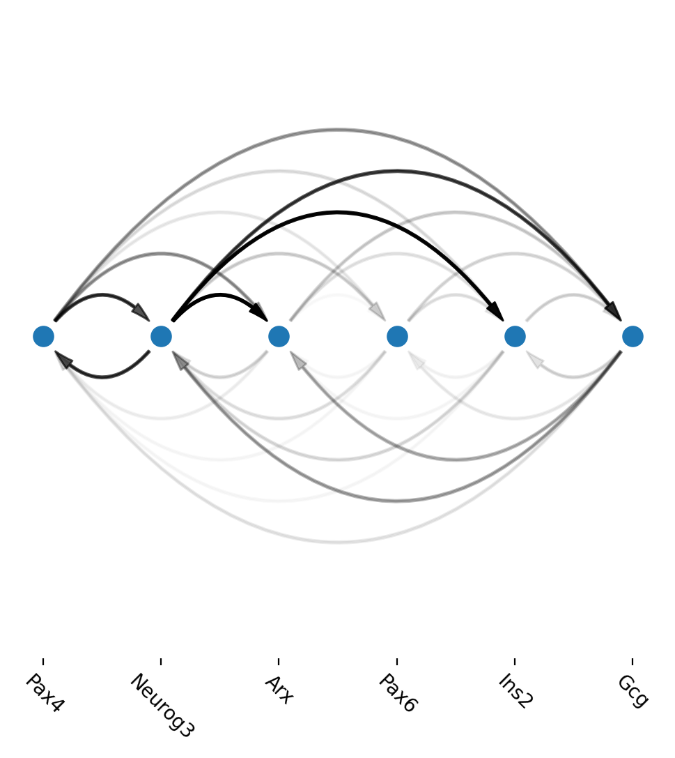
Arcplot shows gene regulatory networks in progenitors and beta cells
Next we use dyn.vf.build_network_per_cluster to build an cluster2edges dictionary which maps cluster name (celltype) to dataframes containing edge information that is necessary to build a networkx graph object. Then we can visualize regulatory networks via dyn.pl.arcPlot.
An example regulatory network in progenitor (Ductal) cells
[21]:
cell_type_regulators = ["Neurog3", "Arx", "Pax4", "Pax6", "Gcg", "Ins2", "Ss5", "Ghri"]
cluster2edges = dyn.vf.build_network_per_cluster(
    adata,
    cluster="clusters",
    cluster_names=None,
    full_reg_rank=full_reg_rank,
    full_eff_rank=full_eff_rank,
    genes=cell_type_regulators,
    n_top_genes=100,
)

import networkx as nx

network = nx.from_pandas_edgelist(
    cluster2edges["Ductal"], "regulator", "target", edge_attr="weight", create_using=nx.DiGraph()
)

ax = dyn.pl.arcPlot(
    adata, cluster="clusters", cluster_name="Beta", edges_list=None, network=network, color=None
)  # color="M_s")
|-----> [iterating reg_groups] in progress: 100.0000%
|-----> [iterating reg_groups] finished [0.1333s]
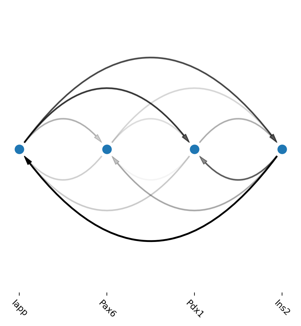
Another example regulatory network in Beta cells
[22]:
cell_type_regulators = ["Pax6", "Pdx1", "Iapp", "Ins2"]
cluster2edges = dyn.vf.build_network_per_cluster(
    adata,
    cluster="clusters",
    cluster_names=None,
    full_reg_rank=full_reg_rank,
    full_eff_rank=full_eff_rank,
    genes=cell_type_regulators,
    n_top_genes=100,
)

import networkx as nx

network = nx.from_pandas_edgelist(
    cluster2edges["Beta"], "regulator", "target", edge_attr="weight", create_using=nx.DiGraph()
)

ax = dyn.pl.arcPlot(
    adata, cluster="clusters", cluster_name="Beta", edges_list=None, network=network, color=None
)  # color="M_s")
|-----> [iterating reg_groups] in progress: 100.0000%
|-----> [iterating reg_groups] finished [0.1114s]
Acceleration Ranking
The acceleration can be computed based on the Jacobian. The acceleration indicates the rate of change in the velocity for a gene.
[23]:
dyn.vf.acceleration(adata, basis='pca')
dyn.vf.rank_acceleration_genes(adata, groups='clusters')
|-----> [Calculating acceleration] in progress: 100.0000%
|-----> [Calculating acceleration] finished [0.1464s]
|-----> <insert> acceleration to layers in AnnData Object.
[23]:
AnnData object with n_obs × n_vars = 3696 × 27998
    obs: 'clusters_coarse', 'clusters', 'S_score', 'G2M_score', 'nGenes', 'nCounts', 'pMito', 'pass_basic_filter', 'Size_Factor', 'initial_cell_size', 'spliced_Size_Factor', 'initial_spliced_cell_size', 'unspliced_Size_Factor', 'initial_unspliced_cell_size', 'ntr', 'cell_cycle_phase', 'pca_ddhodge_div', 'pca_ddhodge_potential', 'divergence_pca', 'control_point_pca', 'inlier_prob_pca', 'obs_vf_angle_pca', 'umap_ddhodge_div', 'umap_ddhodge_potential', 'curl_umap', 'divergence_umap', 'control_point_umap', 'inlier_prob_umap', 'obs_vf_angle_umap', 'speed_pca', 'acceleration_pca', 'jacobian_det_pca'
    var: 'highly_variable_genes', 'nCells', 'nCounts', 'pass_basic_filter', 'log_m', 'log_cv', 'score', 'frac', 'use_for_pca', 'ntr', 'beta', 'gamma', 'half_life', 'alpha_b', 'alpha_r2', 'gamma_b', 'gamma_r2', 'gamma_logLL', 'delta_b', 'delta_r2', 'bs', 'bf', 'uu0', 'ul0', 'su0', 'sl0', 'U0', 'S0', 'total0', 'use_for_dynamics', 'use_for_transition'
    uns: 'clusters_coarse_colors', 'clusters_colors', 'day_colors', 'neighbors', 'pca', 'pp', 'velocyto_SVR', 'PCs', 'explained_variance_ratio_', 'pca_mean', 'pca_fit', 'feature_selection', 'cell_phase_genes', 'dynamics', 'grid_velocity_umap', 'grid_velocity_pca', 'VecFld_pca', 'VecFld_umap', 'clusters_graph', 'jacobian_pca', 'rank_acceleration', 'rank_abs_acceleration'
    obsm: 'X_pca', 'X_umap', 'X', 'cell_cycle_scores', 'velocity_umap', 'velocity_pca', 'velocity_pca_SparseVFC', 'X_pca_SparseVFC', 'velocity_umap_SparseVFC', 'X_umap_SparseVFC', 'acceleration_pca'
    layers: 'spliced', 'unspliced', 'X_spliced', 'X_unspliced', 'M_u', 'M_uu', 'M_s', 'M_us', 'M_ss', 'velocity_S', 'acceleration'
    obsp: 'distances', 'connectivities', 'moments_con', 'pearson_transition_matrix', 'pca_ddhodge', 'umap_ddhodge'
[24]:
adata.uns['rank_acceleration'][:5]
[24]:
| Alpha | Beta | Delta | Ductal | Epsilon | Ngn3 high EP | Ngn3 low EP | Pre-endocrine | |
|---|---|---|---|---|---|---|---|---|
| 0 | Ghrl | Ins1 | Ins1 | Cdc20 | Tmsb4x | Chga | Neurog3 | Tmsb4x |
| 1 | Cck | Ins2 | Cck | Ccnb2 | Gcg | Chgb | Tmsb4x | Pyy |
| 2 | Mdk | Xist | Cdkn1a | Hmgb2 | Nkx6-1 | Tm4sf4 | Btbd17 | Iapp |
| 3 | Rbp4 | Krt8 | Ins2 | Hist1h2bc | Rps19 | Akr1c19 | Mdk | Calr |
| 4 | Serpina1c | Gpx3 | Krt7 | Birc5 | Tmsb10 | Cryba2 | Btg2 | Ppp1r14a |
Enrichment Analysis
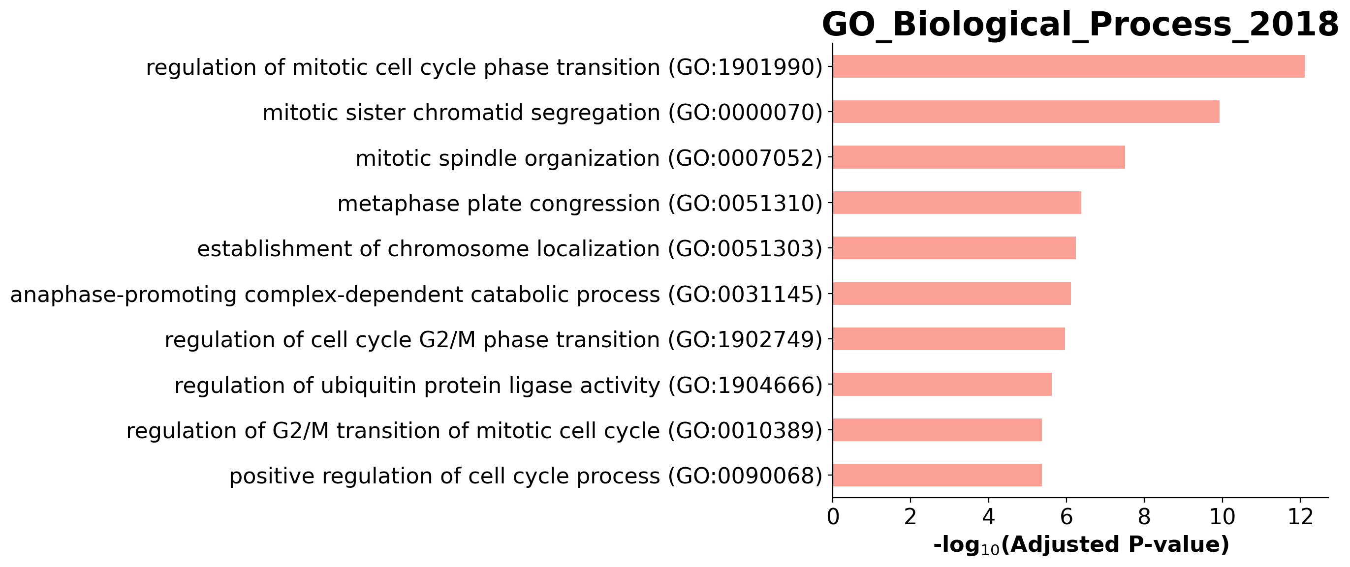
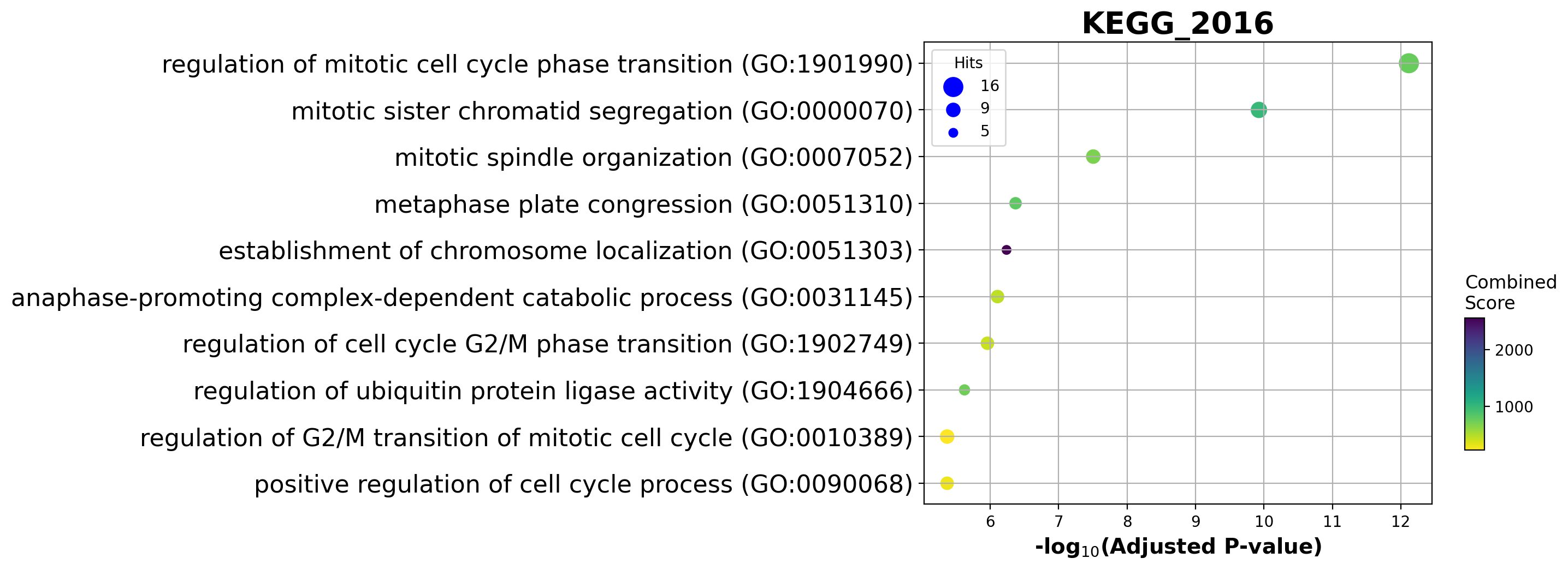
Enrichment analysis allows us to see if top ranking genes are significantly enriched in certain biological pathways. For example, when we pick the top 100 accelerating genes in Ductal cells, we found that they are highly enriched in cell cycle related pathways.
[25]:
enr = dyn.ext.enrichr(adata.uns['rank_acceleration']['Ductal'][:100].to_list(), organism='mouse', outdir='./enrichr')
enr.results.head(5)
[25]:
| Gene_set | Term | Overlap | P-value | Adjusted P-value | Old P-value | Old Adjusted P-value | Odds Ratio | Combined Score | Genes | |
|---|---|---|---|---|---|---|---|---|---|---|
| 0 | GO_Biological_Process_2018 | regulation of mitotic cell cycle phase transit... | 16/184 | 9.341163e-16 | 7.622389e-13 | 0 | 0 | 22.371882 | 774.222174 | HSP90AA1;ANAPC16;NDE1;BUB1B;HMMR;DYNLL1;AURKA;... |
| 1 | GO_Biological_Process_2018 | mitotic sister chromatid segregation (GO:0000070) | 11/82 | 2.897512e-13 | 1.182185e-10 | 0 | 0 | 34.517962 | 996.525054 | CENPE;CCNB1;KIFC1;PRC1;NUSAP1;CDCA8;KIF23;KIF2... |
| 2 | GO_Biological_Process_2018 | mitotic spindle organization (GO:0007052) | 9/74 | 1.142841e-10 | 3.108527e-08 | 0 | 0 | 30.180051 | 690.891800 | CENPE;TPX2;CCNB1;KIFC1;PRC1;BIRC5;KIF23;AURKA;... |
| 3 | GO_Biological_Process_2018 | metaphase plate congression (GO:0051310) | 7/44 | 2.078922e-09 | 4.241002e-07 | 0 | 0 | 40.407149 | 807.796133 | CENPE;CCNB1;CENPF;KIFC1;CDCA8;KIF2C;KIF22 |
| 4 | GO_Biological_Process_2018 | establishment of chromosome localization (GO:0... | 5/13 | 3.521204e-09 | 5.746605e-07 | 0 | 0 | 130.868421 | 2547.283519 | CENPE;CENPF;NDE1;KIF2C;KIF22 |
[26]:
from gseapy.plot import barplot, dotplot
barplot(enr.res2d, title='GO_Biological_Process_2018', cutoff=0.05)
dotplot(enr.res2d, title='KEGG_2016',cmap='viridis_r', cutoff=0.05)
[26]:
<AxesSubplot:title={'center':'KEGG_2016'}, xlabel='-log$_{10}$(Adjusted P-value)'>
[27]:
enr = dyn.ext.enrichr(adata.uns['rank_acceleration']['Ngn3 low EP'][:100].to_list(), organism='mouse', outdir='./enrichr')
enr.results.head(5)
2022-03-12 13:48:23,207 Warning: No enrich terms using library GO_Biological_Process_2018 when cutoff = 0.05
[27]:
| Gene_set | Term | Overlap | P-value | Adjusted P-value | Old P-value | Old Adjusted P-value | Odds Ratio | Combined Score | Genes | |
|---|---|---|---|---|---|---|---|---|---|---|
| 0 | GO_Biological_Process_2018 | purine ribonucleotide metabolic process (GO:00... | 4/66 | 0.000334 | 0.159565 | 0 | 0 | 13.331989 | 106.701278 | TPST2;SULT2B1;ACLY;HSPA8 |
| 1 | GO_Biological_Process_2018 | oxoacid metabolic process (GO:0043436) | 3/32 | 0.000541 | 0.159565 | 0 | 0 | 21.191966 | 159.391414 | TPST2;SULT2B1;SULF2 |
| 2 | GO_Biological_Process_2018 | bone development (GO:0060348) | 3/34 | 0.000648 | 0.159565 | 0 | 0 | 19.822747 | 145.516274 | GNAS;PPIB;SULF2 |
| 3 | GO_Biological_Process_2018 | regulation of protein dephosphorylation (GO:00... | 3/40 | 0.001048 | 0.159565 | 0 | 0 | 16.603232 | 113.917477 | PPP1R14A;PPP1R14B;CALM2 |
| 4 | GO_Biological_Process_2018 | positive regulation of nuclear-transcribed mRN... | 2/11 | 0.001322 | 0.159565 | 0 | 0 | 45.104308 | 298.984305 | BTG2;TOB1 |